


ABSTRACT
We explore the variation in single-star 15–30  , nonrotating, solar metallicity, pre-supernova MESA models that is due to changes in the number of isotopes in a fully coupled nuclear reaction network and adjustments in the mass resolution. Within this two-dimensional plane, we quantitatively detail the range of core masses at various stages of evolution, mass locations of the main nuclear burning shells, electron fraction profiles, mass fraction profiles, burning lifetimes, stellar lifetimes, and compactness parameter at core collapse for models with and without mass-loss. Up to carbon burning, we generally find that mass resolution has a larger impact on the variations than the number of isotopes, while the number of isotopes plays a more significant role in determining the span of the variations for neon, oxygen, and silicon burning. Choice of mass resolution dominates the variations in the structure of the intermediate convection zone and secondary convection zone during core and shell hydrogen burning, respectively, where we find that a minimum mass resolution of ≈0.01
  is necessary to achieve convergence in the helium core mass at the ≈5% level. On the other hand, at the onset of core collapse, we find ≈30% variations in the central electron fraction and mass locations of the main nuclear burning shells, a minimum of ≈127 isotopes is needed to attain convergence of these values at the ≈10% level.
Export citation and abstract BibTeX RIS
1. INTRODUCTION
The end evolutionary phases of massive stars remain a rich site of fascinating challenges that include the interplay between convection (Meakin & Arnett 2007b; Viallet et al. 2013), nuclear burning (Couch et al. 2015), rotation (Heger et al. 2000; Rogers 2015; Chatzopoulos et al. 2016), radiation transport (Jiang et al. 2015), instabilities (Garaud et al. 2015; Wheeler et al. 2015), mixing (Maeder & Meynet 2012), waves (Rogers et al. 2013; Aerts & Rogers 2015; Fuller et al. 2015), eruptions (Humphreys & Davidson 1994; Kashi et al. 2016), and binary partners (Justham et al. 2014; Marchant et al. 2016). This bonanza of physical puzzles is closely linked with compact object formation by core-collapse supernovae (SNe) (Timmes et al. 1996; Eldridge & Tout 2004; Özel et al. 2010) and the diversity of observed massive star transients (e.g., Van Dyk et al. 2000; Ofek et al. 2014; Smith et al. 2016). Recent observational clues that challenge conventional wisdom (Zavagno et al. 2010; Vreeswijk et al. 2014; Boggs et al. 2015; Jerkstrand et al. 2015; Strotjohann et al. 2015), coupled with the expectation of large quantities of data from upcoming surveys (e.g., Creevey et al. 2015; Papadopoulos et al. 2015; Sacco et al. 2015; Yuan et al. 2015), new measurements of key nuclear reaction rates and techniques for assessing reaction rate uncertainties (Iliadis et al. 2011; Wiescher et al. 2012; Sallaska et al. 2013), and advances in three-dimensional (3D) pre-supernova (pre-SN) modeling (Couch et al. 2015; Jones et al. 2016; Müller et al. 2016) offer significant improvements in our quantitative understanding of the end states of massive stars.
One end state, a core-collapse supernova (SN), is the result of another end state, that of massive star progenitors undergoing gravitational collapse (e.g., Sukhbold & Woosley 2014; Perego et al. 2015; Sukhbold et al. 2016). The amount of mass of an isotope that can be injected into the interstellar medium (e.g., Woosley & Weaver 1995; Limongi & Chieffi 2003; Nomoto et al. 2013) depends on the structure of the star at the point of core collapse. In turn, the pre-SN structure depends on the evolutionary pathway taken by the massive star during its lifetime (e.g., Nomoto & Hashimoto 1988; Jones et al. 2013).
This paper is novel in two ways. First, we scrutinize the structure and evolution of single massive stars from the pre-main sequence (pre-MS) to the onset of core collapse with multiple, possibly large, in situ nuclear reaction networks. For the first time, we quantify aspects of the structure and evolution that are robust, or can be made robust, with respect to variations in the nuclear reaction network used for the entire evolution. For example, we explore the diversity of pre-SN model properties such as the mass locations of the major burning stages, core masses at various stages of evolution, mass fraction profiles, and electron fraction profiles. Second, for each nuclear reaction network we investigate the impact of methodically and systematically changing the mass resolution on the structure and evolution of a set of massive stars.
In Section 2 we discuss the software instruments, input physics, reaction networks, and model choices. In Section 3 we present the results for different reaction networks, and mass resolutions with and without mass-loss. In Section 4 we discuss our results and their implications.
2. STELLAR MODELS
Models of 15, 20, 25, and 30  are evolved using the Modules for Experiments in Stellar Astrophysics software instrument (henceforth MESA , version 7624, Paxton et al. 2011, 2013, 2015). All models begin with a metallicity of Z = 0.02 and a solar abundance distribution from Grevesse & Sauval (1998). The models are evolved without mass-loss or with the "Dutch" wind-loss scheme (Nieuwenhuijzen & de Jager 1990; Nugis & Lamers 2000; Vink et al. 2001; Glebbeek et al. 2009) with an efficiency η = 0.8 for these nonrotating models (Maeder & Meynet 2001). Each stellar model is evolved from the pre-MS until core collapse, which we take as the time when any location inside the stellar model reaches an infall velocity of 1000
  . To compute the infall velocity, we set MESA's v_flag=.true., which adds a hydrodynamic radial velocity term to the model. This additional variable is evolved from the zero-age main sequence (ZAMS) until core collapse, although it only becomes relevant to the evolution after core oxygen-burning.
All the MESA inlists and many of the stellar models are publicly available.6
2.1. Mass and Temporal Resolution
MESA provides several controls to specify the mass resolution of a model. Sufficient mass resolution is required to accurately determine gradients of stellar structure quantities, but an excessive number of cells impacts performance. One parameter for changing the mass resolution in regions of rapid change is mesh_delta_coeff ( ), which acts a global scale factor limiting the change in stellar structure quantities between two adjacent cells. Lower values of
  increase the number of cells. Another parameter controlling mass resolution is the maximum fraction of a star's mass in a cell, max_dq. That is, the minimum number of cells in a stellar model is 1/max_dq. We use
  and
and  , where
  is the mass of the stellar model in solar mass units at time τ and
  is a parameter we vary between 0.1
  and 0.005
  . We choose to vary max_dq instead of mesh_delta_coeff to enable us to set a minimum level of mass resolution in the model.
MESA also offers a rich set of timestep controls. The parameter  broadly controls the temporal resolution by modulating the magnitude of the allowed changes between individual timesteps. At a finer level of granularity, dX_nuc_drop_limit limits the maximum allowed change of the mass fractions between timesteps for mass fractions larger than dX_nuc_drop_min_X_limit. We use
  = 5 × 10⁻⁵, dX_nuc_drop_limit = 10−3, and dX_nuc_drop_min_X_limit = 10−3 for the evolution between the pre-MS to the onset of core Si-burning, where we loosen the criteria to allow larger timesteps;
  = 5 × 10⁻⁵, dX_nuc_drop_limit = 5 × 10⁻², and dX_nuc_drop_min_X_limit = 5 × 10⁻².
The timestep control delta_lg_XH_cntr_min regulates the time step as hydrogen is depleted in the core, which aids in resolving the transition from the ZAMS to the terminal-age main sequence (TAMS). Similarly, the timestep controls delta_lg_XHe_cntr_min, delta_lg_XC_cntr_min, delta_lg_XNe_cntr_min, delta_lg_XO_cntr_min, and delta_lg_XSi_cntr_min control the timestep as one of the major fuels is depleted in the core. These timestep controls are useful for obtaining, for example, convergence of mass shell locations, smoother transitions as a stellar model exits core H-burning in the HR diagram (i.e., the "Henyey Hook," Kippenhahn et al. 2012), and smoother trajectories in the central temperature  -central density
  plane. We use a mass fraction value of 10−6 for all these fuel depletion timestep controls. Additionally, we use MESA's default timestep controls for controlling changes in the hydrodynamics. At the point where hydrodynamics becomes important, during Si-burning, we find we are limited by the delta_lg_XSi_cntr_min control rather than by changes in the hydrodynamics.
2.2. Nuclear Reaction Networks
MESA evolves models of massive stars from the pre-MS to the onset of core collapse with the nuclear burning fully coupled to the hydrodynamics using a single, possibly large, reaction network (see Paxton et al. 2015). This capability avoids the challenges of (a) operator splitting errors from evolving the hydrodynamics and nuclear burning independently; (b) stitching together different solution methods for different phases of evolution, for example, combining a reaction network with equilibrium methodologies such as quasi-static equilibrium (QSE) or nuclear statistical equilibrium (NSE), or with the use of an adaptive network that modifies itself based on the most populous isotopes present; or finally, (c) evolving a stellar model with a small reaction network while carrying along a larger reaction network that does not impact the energy generation rate or composition of the stellar structure, i.e., passive coprocessing. MESA's unified approach is not just a solution to issues of accuracy or self-consistency. It offers an improvement by providing a single-solution methodology—in situ reaction networks evolved simultaneously with the hydrodynamics.
We evolve each stellar model with one of the five nuclear reaction networks shown in Figure 1. We consider a small network, approx21_cr60_plus_co56.net (hereafter approx22.net), where each reaction pathway has been predetermined (i.e., a "hardwired" network). Such approximate networks, an α-chain backbone with aspects of H-burning, heavy ion reactions, and iron-group photodisintegration, are a traditional workhorse in massive star models (e.g., Weaver et al. 1978; Woosley & Weaver 1988; Heger et al. 2000; Heger & Woosley 2010; Chatzopoulos & Wheeler 2012). We also use four "softwired" networks, where after specifying the isotopes, all allowed reaction pathways between the isotopes are linked. Specifically, we consider mesa_79.net, which contains isotopes up to 60Zn (black dots); mesa_127.net, which adds neutron-rich isotopes in the iron group (purple crosses); mesa_160.net, which adds more neutron-rich isotopes and a few proton-rich isotopes (green squares); and mesa_204.net, which adds isotopes lighter than 36Cl (black squares), and includes the isotopes identified in Heger et al. (2001) as important for the electron fraction,  , in core-collapse models.

Figure 1. The five reaction networks used to quantify the variance of the properties of the pre-SN cores as a function of the number of isotopes in a network.
Download figure:
Standard image High-resolution imageThe softwired reaction networks are designed to yield approximately the same final  as a 3298 isotope reaction network in one-zone burn calculations of the thermodynamic history of 15
  cores (Paxton et al. 2015). For example, in one-zone burn calculations the mesa_204.net reaction network gives a final
  , while the 3298 isotope reaction network gives
  .
.
All forward thermonuclear reaction rates are from the JINA reaclib version V2.0 2013-04-02 (Cyburt et al. 2010). Inverse rates are calculated directly from the forward rates (those with positive Q-value) using detailed balance, rather than using fitted rates. The nuclear partition functions used to calculate the inverse rates are from Rauscher & Thielemann (2000). Electron screening factors for both weak and strong thermonuclear reactions are from Alastuey & Jancovici (1978) with plasma parameters from Itoh et al. (1979). All the weak rates are based (in order of precedence) on the tabulations of Langanke & Martínez-Pinedo (2000), Oda et al. (1994), and Fuller et al. (1985). Thermal neutrino energy losses are from Itoh et al. (1996).
2.3. Mixing
We treat convection using the mlt++ approximation (Paxton et al. 2013). This prescription takes the convective strength as computed by mixing length theory (MLT) and reduces the superadiabaticity in radiation dominated convection zones (e.g., near the iron opacity peak). This decreases the temperature gradient in these regions, and the artificial suppression can be viewed as treating additional, unmodeled, energy transport mechanisms in these regions (e.g., Jiang et al. 2015). Values of  have been inferred from comparing observations with stellar evolution models (Noels et al. 1991; Miglio & Montalbán 2005; Aerts et al. 2010), and 3D hydrodynamic simulations of the deep core and surface layers also suggest a similar range (Viallet et al. 2013; Trampedach et al. 2014; Jiang et al. 2015). These efforts inform our baseline choice of
  = 1.5, although this is by no means the only choice (Dessart et al. 2013).
Convective overshooting is assumed to be an exponential decay beyond the Schwarzschild boundary of convection (Herwig et al. 1997). The convective diffusion coefficient,  , is measured at a distance
  inside the convection zone. Overshooting then extends beyond the edge of the convection zone a fraction
  of the local pressure scale height
  ,
,

where  is the overshooting diffusion coefficient at a radial distance z from the edge of the convection zone boundary. Our baseline choices for the overshoot mixing are
  and
and  . This choice is motivated by recent calibration of a 1D 25
  pre-SN model to idealized 3D hydrodynamic simulations of turbulent O-burning shell convection (Jones et al. 2016). MESA offers the flexibility to have different values for convection driven by different types of nuclear burning (H, He, C, and others) and whether the burning occurs near the core or in a shell, but for simplicity, we take these values to be the same for all regions.
Thermohaline mixing is included in the models when  , where B is the Brünt composition gradient. The thermohaline mixing diffusion coefficient
  is parameterized as

where  is a dimensionless parameter, K is the radiative conductivity, and
  is the specific heat at constant pressure (Ulrich 1972; Kippenhahn et al. 1980). Continuing attempts to calibrate
  include multidimensional simulations of fingering convection under stellar conditions (Traxler et al. 2011; Brown et al. 2013; Garaud et al. 2015). We set
  = 2.0 except during core silicon burning, where we set
  = 0.0.
Finally, we include semiconvection when  , where
  . We take the strength of semiconvective mixing
  as Langer et al. (1983) and Langer et al. (1985),

where  is a dimensionless parameter. Ongoing efforts to calibrate 1D semiconvection models include multidimensional simulations of double diffusive convection (Spruit 2013; Zaussinger & Spruit 2013) and comparing massive star models with observations (Yoon et al. 2006). While recent work suggests that to a first-order approximation, the effect of semiconvection can be neglected (Moll et al. 2016), we adopt a baseline choice of
  .
.
3. RESULTS
We present the variations in the MESA version 7624 pre-SN model properties that are due to changes in the nuclear reaction network and mass resolution in the order of the major burning stages; H-burning in Section 3.1, stellar lifetimes in Section 3.2, He-burning in Section 3.3, C-burning in Section 3.4, Ne-burning in Section 3.5, O-burning in Section 3.6, Si-burning in Section 3.7, the onset of core collapse in Section 3.8, and representative pre-SN nucleosynthesis yields in Section 3.9.
3.1. Core/Shell H-burning
Figure 2 shows the MS and giant branch (GB) evolution of a 15  model at two resolutions
 and
and 
 , evolved without mass-loss and with the approx22.net network. As stars evolve off of the pre-MS and onto the ZAMS, they begin burning hydrogen in a convective core, predominantly via the CNO cycle, but also via primordial 3He in the pp chain (Hansen et al. 2004; Iben 2013a, 2013b). This convective region expands outwards to consume approximately half the mass of the star. Once the primordial 3He is exhausted, at
  in Figure 2, the convection region recedes and the core temperature and density increase. At this point in the evolution, most of the primordial 12C is already piled up in 14N as a result of the proton capture onto 14N reaction rate (Arnett 1996; Iliadis 2007). Owing to the strong temperature dependence of the CNO cycle, the energy production increases and the convective region expands slightly farther out in mass coordinate than the first peak at
  . The increased energy generation from the CNO cycle causes the star itself also to begin expanding at this point.

Figure 2. Kippenhahn plot for a solar metallicity 
 model evolved with the approx22.net and without mass-loss. The left panel shows a mass resolution of
 , the right panel a mass resolution of
 . The age shown on the x-axis is the time until convection begins in core He-burning, set such that the SCZ can be temporally resolved. Yellow to red regions denote logarithmic increases in the net nuclear energy generation rate. Blue marks convective regions, gray identifies overshoot regions, purple designates semiconvective regions, and green labels thermohaline mixing regions. Labeled are the intermediate convection zone (ICZ), secondary convection zone (SCZ), H-core, H-shell, and He core. The inset Kippenhahn diagram shows the behavior of the convective core during the transition between 3He and CNO burning.
Download figure:
Standard image High-resolution imageThe convective core shrinks during core H-burning. This recession leaves behind a composition gradient (μ-gradient,  ) and lower levels of nuclear burning. Our models form a layered structure of semiconvective and convective regions, labeled an intermediate convection zone (ICZ) in Figure 2, at
  at the approximate mass coordinate of the maximal extent of the core convection zone (≈6
  ) (Langer et al. 1985; Heger et al. 2000; Hirschi et al. 2004). As the mass resolution or the initial mass of the stellar model increases, the structure and behavior the ICZ changes. For the
 models, in Figure 2, when the mass resolution is increased from
 to
to 
 , the fraction (in mass coordinates) of semiconvection in the ICZ decreases while the amount of convection increases.
Figure 2 shows that as the mass resolution increases the fine structure of the H-core convection zone, the maximal extent of the H-core extent and the edge of the overshoot region are better determined. All of which determine how much fresh H fuel is pulled into the core during the MS and how much fuel is available just outside the convective core to form the ICZ. At higher resolution less hydrogen is burned when the ICZ forms, which makes the star more compact as a consequence of the decreased burning. As less hydrogen has been burned,  is smaller.
Semiconvection occurs when  where
where  is a function of
  . When
  is large enough, it can maintain a semiconvective region over the entire ICZ. If
  is small in a local region, then the semiconvective region may transition into a convective region (Langer et al. 1985). This occurs in Figure 2 in the higher resolution
 panel where
  is smaller, allowing more convection to develop inside the semiconvective region (Mowlavi & Forestini 1994). This is most clearly seen as the bifurcation of the ICZ in the lower resolution
 (left panel), while in the right panel the convection zone is embedded inside the semiconvective region. Higher mass resolutions also capture the substructure in the
  , which become the seeds for the convective regions to form.
Langer et al. (1985) showed similar variations in the ICZ structure by varying the strength of the  parameter. As the efficiency of semiconvection increases, the fine structure increases. Our MESA models achieve a similar result by varying the mass resolution for a fixed
  .
.
A secondary convective zone (SCZ) then forms at  in both models, when H-shell burning begins. Figure 2 shows how the structure and behavior of the SCZ change with mass resolution. The low-resolution model (left panel) has layered semiconvection/convection that stays outside of the H-shell. In the higher resolution model (right panel), the SCZ is dominated by convection that propagates into the H-shell burning region. This merger of the SCZ and the H-shell leads to fresh fuel being injected into the H-shell and allows the star to live longer. If the star has mass-loss, then the longer H-burning lifetimes create larger He-cores that will last longer and thus increase the amount of mass lost (Section 3.2).
This difference in behavior arises because the SCZ forms within the mass coordinates previously occupied by the ICZ semiconvective/convective mixing region. The larger convectively mixed region during the ICZ in the higher resolution model implies that the μ-gradient left behind by the receding H-core is reduced or even zero. In turn, this reduction in the μ-gradient allows convection to form over a larger mass range in the SCZ. That is, a preceding semiconvective phase is not necessary to reduce the μ-gradient. This is shown in Figure 2 by the relative difference in mass covered by semiconvection and convection at  .
.
The 
 models without mass-loss are qualitatively similar, and Figure 3 shows a representative set of MESA models. When the ICZ forms, multiple layers of alternating semiconvection and convection form (Langer et al. 1985). At lower mass resolutions (left panel), this structure begins at
 and propagates inwards to
 . As the mass resolution increases (right panel), the convective fingers start at a similar mass coordinate, but will propagate deeper into the star. Figure 3 shows an example of the fingers moving sufficiently inward to penetrate the H-burning core. There is a brief increase in the nuclear burning, as shown by the near step function in burning at
  that arises because the ICZ injects unburnt hydrogen into the core. This leads to a longer MS lifetime for these models. This penetration of the core is a binary process, either the ICZ penetrates the core or it does not. Thus, one may expect step functions in the MS lifetime (Section 3.2).

Figure 3. Same as Figure 2, but for a solar metallicity 
 model evolved with the mesa_79.net and without mass-loss. The left panel is for a mass resolution of
 , and the right panel is for a mass resolution of
 . As convection never ceases in the core, the x-axis is set such that it has a similar scale as Figure 2, and is measured until an arbitrary point during core helium burning.
Download figure:
Standard image High-resolution imageFor the 
 models with mass-loss, Figure 4 shows a third possible state. As the mass resolution increases the SCZ, which formed at the TAMS, it decreases in extent. The left panel of Figure 4 shows that for a relatively coarse mass resolution of
 , the SCZ forms multiple convection/semiconvection zones out to
 , while the right panel shows that for a finer mass resolution of
 , the SCZ forms a single convection zone out to
 . The increased extent of the SCZ region allows more hydrogen fuel to be mixed inwards toward the core, and increases the hydrogen mass fraction by a few percent at the H-burning shell. This allows the H-shell to burn more energetically and for longer. Thus we would expect the models with lower spatial resolution to evolve slower to core collapse, but this effect is limited because of the small change in hydrogen mass fraction.

Figure 4. Same as Figure 2, but for a solar metallicity 
 model evolved with the mesa_127.net and mass-loss. The left panel corresponds to a mass resolution of
 , while the right panel corresponds to a mass resolution of
 . The age shown on the x-axis is the time until convection begins in the He core. Note the change in color-bar scale between the left and right panels; lower mass resolution models release more energy during H-shell burning.
Download figure:
Standard image High-resolution image3.2. Stellar Lifetimes
Figure 5 shows the lifetime for models without mass-loss (top panel) and for models with mass-loss (bottom panel). The most striking feature is the sharp bifurcation of the lifetimes as a function of mass resolution, most prominently seen in the 
 and 30
  models without mass-loss at a spatial resolution of
 . This is a direct consequence of the differences in behavior of the ICZ and SCZ during the MS and GB phases. Models where the ICZ penetrates the MS H-core, or where the SCZ penetrates the H-shell as in the 15
  models, live up to ≈5% longer because fresh hydrogen fuel is injected. Hatching indicates models that do not reach core collapse, although all reach at least Si-burning. Thus we include them in our comparisons up to Si-burning.

Figure 5. Lifetimes in mega years till core collapse as a function of mass resolution and number of isotopes in the nuclear reaction network. Top panel: models without mass-loss; bottom panel: models with mass-loss. Hatching indicate models that did not reach core collapse, but do reach silicon burning.
Download figure:
Standard image High-resolution imageStellar models with and without mass-loss have similar ages, with a trend for stars with mass-loss to have shorter lifetimes (e.g., El Eid et al. 2004). The spread in age is larger for models without mass-loss than for those with mass-loss. This is chiefly due to differences in the size of the timesteps, thus this is a numerical artifact. While all models have the same temporal control  , models with mass-loss require a smaller timestep to keep the variation per step within the limits specified by
  . Smaller timesteps allow the mass lost to be treated more accurately, as the amount of mass-loss per step depends on the stellar parameters at the start of the step, thus smaller timesteps will better capture fast changes in the star's structure.
Compared to the pre-SN lifetimes from Paxton et al. (2011), Limongi et al. (2000), Woosley et al. (2002), and Hirschi et al. (2004), we find in general that the total stellar lifetimes considered agree to within  . The models of Woosley et al. (2002) tend to predict longer lifetimes. Specifically, for the
 model, they predict an
  longer lifetime until core collapse. This value increases to
  for the
 model. Limongi et al. (2000) predict shorter lifetimes with
  difference for their
 model. The models of Paxton et al. (2011) and Hirschi et al. (2004) agree with our values to within
  for
for  and 20
  models, and spread to ±2% for
 . Each set of pre-SN models considered here for comparison uses a slightly differing set of input physics. For example, our models use a more efficient value for convective overshoot than that in the Paxton et al. (2011) models and considers larger nuclear reaction networks. In addition, each set of pre-SN models considered uses different (and often unspecified) mass and temporal resolutions. We find considerable agreement among the total stellar lifetimes, with the largest discrepancies occurring at
 .
.
Models with the same mass resolution show little variation in the final age with respect to changes in the number of isotopes in the reaction network. For example, the 
 models with and without mass-loss in Figure 5 show uniformity in the stellar age as a function of network size on either side of the bifurcation point. This is due to efficient mixing of the composition by convection; it does not make much difference where or when the SCZ penetrates the H-shell, for once it does, the H-shell is injected with similar amounts of fresh fuel (see Figure 2). As the initial mass of the stellar model increases, the magnitude of the spread in the stellar lifetime decreases. This is due to smaller variations in when and where the ICZ penetrates the H-core.
There are outlier models for the smallest network, approx22.net: the 
 model without mass-loss and
 , the
, the 
 model without mass-loss and
 , and the
 model with mass-loss and
 . These are caused by the SCZ penetrating deep into the star, from the edge of the H-burning shell to the radiative region at the center of the star. This injects enough unburnt hydrogen to prolong the lifetimes.
The 
 models without mass-loss in Figure 5 show a lifetime bifurcation at a finer spatial resolution of
 than the
 . In addition, the
 models with mass-loss show the bifurcation is inverted—increasing resolution decreases the stars lifetime—as a result of the relative extent of the SCZ region discussed for Figure 4.
For the 
 and 30
  models, Figure 5 shows that the lifetime bifurcation point varies depending on whether or not there is mass-loss. The stars without mass-loss bifurcate at
 and
and 
 , respectively, while the mass-losing models bifurcate at
 and
and 
 , effectively one level of resolution higher. This variation may be due to our grid of mass resolutions being insufficient to resolve the bifurcation.
We encourage careful consideration of the mass resolution when modeling massive stars with MESA. Not only to the choice MESA's  parameter, which only increases the number of zones if MESA detects a large enough spatial gradient, but also the number of zones used throughout the model. Much of the variation seen in the MS and GB phases is set by the stellar structure at the start of the MS, which is early enough that
  may not have sufficient time to act. From Figures 5 and for our choice of
  , we recommend a mass resolution of at least
 , which equates to at least
  mass cells during the pre-MS and MS evolution in order to reasonably resolve the ICZ and SCZ features. In addition, we recommend temporal controls that limit the timestep as major fuels are depleted in the core (see Section 2.1).
3.3. Core He-burning
Figure 6 shows the He-core mass at the onset of convective core He-burning as a function of mass resolution  and the number of isotopes in the nuclear reaction network. We define the He-core mass as the location where
  and
and  and measured when the star reaches the base of the GB. They share many of the same features—bifurcations and outliers—discussed for the stellar lifetimes in Figure 5. For the
 models without mass-loss the initial He-core mass ranges from ≈2.79 to 2.81
  , while models with mass-loss span ≈2.72–2.77
  . For the
 models without mass-loss the initial He-core mass range between ≈4.6 and 4.7
  , while models with mass-loss span between ≈4.5 and 4.6
  . Our
. Our 
 models without mass-loss show initial He-core mass ranges of ≈6.8 to 7.2
  , while models with mass-loss span ≈6.54–6.66
  . The
. The 
 models without mass-loss show the initial He-core mass ranges between ≈9.2 and 9.8
  , while models with mass-loss span ≈8.63–8.78
  . In general, a longer core H-burning phase produces a higher He-core mass. The initial He-core masses in Figure 6 and their range as a function of mass resolution and number of isotopes in the reaction network are commensurate with the He-core masses found in numerous studies (e.g., Nomoto & Hashimoto 1988; Langer 1991; Wellstein & Langer 1999; Woosley et al. 2002; Petermann et al. 2015; Choi et al. 2016).

Figure 6. The 4He core mass at the formation of the He core, defined as where  and
and  . Top panel: MESA models without mass-loss; bottom panel: models with mass-loss.
Download figure:
Standard image High-resolution imageFigure 7 shows the evolution of the central helium mass fraction,  , during the core He-burning phase of the 20
  models without mass-loss. These central abundances, due to convective mixing, also represent the mass fraction values over the entire He-burning core. The core of these stars begin with
  and
and  and, after ≈106 yr, end with
  and
and  , with the remainder being mostly 12C.

Figure 7. Mass fraction of 4He as a function of time during core He-burning for the 
 models without mass-loss. Left panel: models as a function of the number of isotopes for a fixed resolution of
 . Right panel: models as a function of mass resolution for a fixed approx22.net network. The insets show a zoom-in when
  .
.
Download figure:
Standard image High-resolution imageThe left panel of Figure 7 shows the evolution of  as a function of the number of isotopes in the nuclear reaction network, at a mass resolution of
 for the
 models without mass-loss. The slopes of the lines show that the models are evolving at similar rates. The positive offset in the mesa_204.net is caused by the core being slightly cooler at the start of core helium convection; for the approx22.net the temperature is 177 × 106 K and for mesa_204.net it is 175 × 106 K. Nevertheless, the mesa_204.net model reaches
  at the same time as the other models. The spikes in
  for the small approx22.net, expanded in the inset plot, are due to core breathing pulses (henceforth CBP, see Castellani et al. 1985). These occur when the
  value is low, such that if the core convection expands slightly outwards in mass, then a small entrainment of unburnt 4He leads to a large increase in the nuclear energy production (Straniero et al. 2003). For the approx22.net models, the edge of the convection core can move inwards and outwards ≈0.5
  on timescales of ≈200 yr. The models with larger nuclear networks have significantly smaller CBPs as their convection cores move inwards and outwards ≈0.05
  , entraining a significantly smaller amount of additional 4He fuel.
The left panel of Figure 7 shows that the approx22.net almost doubles  during a CBP. The nuclear energy generated from a CBP is sufficient to expand the stellar envelope, which can be seen as a blue loop in theoretical HR diagrams (e.g., Constantino et al. 2016). The impact of a CBP is also mirrored in the evolution of
  , and leads to a larger
  at the end of core He-burning and thus a smaller 12C mass fraction. All these models at constant
  have between 1600 and 1700 zones and a similar timestep distribution at this evolutionary stage, thus the differences between CBPs are not due to changes in resolution. The presence of CBPs has been suspected as being a numerical artifact (Caputo et al. 1989; Boothroyd et al. 1993; Constantino et al. 2016), and we show that it can also be due to the choice of the nuclear network.
The right panel of Figure 7 shows the evolution of  as a function of mass resolution for approx22.net. There is a wide variation in
  . The
. The 
 and
and 
 models both have CBPs, with the
 models starting their CBPs at earlier times with a larger
  . This reinforces the notion that these approx22.net CBPs are purely numerical artifacts. Increasing the resolution above
 (which is also necessary for the ICZ to penetrate the H-core) is sufficient to prevent the CBP from forming. Models with CBPs have between 1500 and 2000 zones, while models without CBP have between 2000 and 7000 zones.
During core He-burning, the convective core grows, largely because the mass of the He core itself grows from the overlying H-burning shell. This growth of the He core has two effects. First, as the mass of the He core grows, so does the core luminosity, but the radius of the convective core stays nearly the same. This causes the density of the core to steadily increase as core He-burning proceeds. Second, as the mass of the He core rises, the ratio of the gas pressure to the total pressure decreases, which favors efficient convection in the core.
The core prior to C-ignition is composed of the ashes of core He-burning, mainly 12C and 16O in a ≈1:4 ratio for the choice of 12C( )16O reaction rate from the JINA reaclib version V2.0 2013-04-02 (see Figure 7, and West et al. 2013). There are also other isotopes present in trace amounts such as the neutron-rich
  Ne,
Ne,  Mg from processing the ashes of the CNO elements during He-burning; about 1% of X(20Ne) from 16O(
 )20Ne during He-burning; the light s-process (which we do not follow); and other heavy elements present since the pre-MS from the initial composition.
Figure 8 shows the 4He mass fraction profile during C-burning for a subset of the 
 models. The left panel plots the X(4He) profile as a function of the number of isotopes in the network for the models without mass-loss and a mass resolution of
 . The inset plot is a zoom-in of the inner edge of the He shell. We find that the inner and outer mass location of the He shell agree within
 across all network sizes. The right panel plots the X(4He) profile as a function of mass resolution for the models without mass-loss, which use the largest reaction network considered, mesa_204.net. The inset plot is a zoom of the inner edge of the He shell. We find that mass resolutions of
  and 0.05
  do not sufficiently resolve the He-burning shell locations. For mass resolutions
 , we find convergence of the He shell inner and outer boundaries.

Figure 8. 4He mass fraction profile at the onset of C-burning for the 
 model without mass-loss as a function of (a) the number of isotopes in the nuclear reaction network and (b) the mass resolution
Download figure:
Standard image High-resolution image3.4. C-burning
Figure 9 shows the C-core mass at the onset of C-burning as a function of mass resolution and the number of isotopes in the nuclear reaction network. The core mass is defined as the mass location where  and
and  , measured when the core reaches
  . These maps share many of the same variations, chiefly the bifurcations and outliers, that are inherited from core H-burning (see Figure 5). For the
 models without mass-loss, the initial C-core mass is in the range
 , while models with mass-loss span
 . The
. The 
 models without mass-loss have initial C-core masses spanning
 , while models with mass-loss span
 . Our
. Our 
 models without mass-loss show initial C-core masses of
 , while models with mass-loss span
 . The
. The 
 models without mass-loss have an initial C-core mass range of
 , while models with mass-loss span
 .
.

Figure 9. Carbon core mass at carbon ignition as a function of the number of isotopes in the network and mass resolution. Top: for MESA models without mass-loss. Bottom: for models with mass-loss.
Download figure:
Standard image High-resolution imageWhen we compare this with Figure 6, the 
 models with initially more massive He core have less massive C-cores at carbon ignition. This is because less massive ZAMS models have a larger electron degeneracy in the C-core, a larger
  , and thus an enhanced screening factor for the 12C+12C reaction rate. For models more massive than the
 , those with larger He-cores have the largest C-core at carbon ignition.
All the 
 models undergo convective C-ignition at the center of the star followed by a series of three convective flashes, where each additional flash ignites at the approximate maximum mass location of the previous convective C-flash. All the
 and 30
  models show C-ignition under radiative conditions. This ignition propagates outwards in mass, followed by a single convective flash. The
 models have a more complex C-ignition that straddles the boundary between radiative and convective carbon burning (Timmes et al. 1996; Heger et al. 2000; Hirschi et al. 2004).
Figure 10 shows the differences in core C-ignition for the 
 model without mass-loss and with the mesa_160.net network. As the mass resolution increases, C-ignition transitions from radiative conditions at the coarsest resolution (
 ) to a mixture of convective and radiative conditions at intermediate resolutions (
 ), and finally to purely convective conditions at higher resolutions (
 ). Models with yet finer mass resolution are similar to the
 case.
case.

Figure 10. Kippenhahn plots for the 
 models without mass-loss and the mesa_160.net reaction network. The top left panel shows
 , the top right panel
 , and the bottom panel
 . Time is measured in years until core collapse. Red/orange regions denote vigorous burning, while purple denotes significant cooling and electron degeneracy. Regions with convection are plotted in light blue, regions with convective overshoot are shown in gray, and regions with semiconvection are presented in purple; thermohaline mixing is not shown for clarity. At the coarsest resolution (top left), carbon burns under radiative condition with one convective episode. At finer resolution (top right), carbon ignites under radiative/convective conditions followed by two convective flashes, while at the higher resolutions (bottom), C-ignition occurs under convective conditions with three episodes of convective C-burning.
Download figure:
Standard image High-resolution imageCarbon burning in all cases begins at the center. In the case of the 
 model with the coarsest resolution shown in Figure 10, the central temperature is high enough (
 ) to burn carbon even though the central regions are still dominated by thermal neutrino cooling (light purple). Only near
 at
at  ≈ 1.7 does the nuclear energy generation rate from burning overtake the thermal neutrino cooling rate, and thus the color in the Kippenhahn transitions to red.
As the C-ignition conditions transition from radiative to convective, the time spent in the core C-burning phase increases from ≈45 to ≈250 yr. After carbon burning ceases, the star has  year until core collapse. As the mass resolution increases, the mass location of the innermost boundary of the 4He shell (see Figure 8) decreases, while the mass location of the outer boundary of the 12C shell increases by
 . In addition, as the resolution increases,
  decreases from 8.90 to 8.88 and log10 (
 /(g cm−3)) decreases from 5.36 to 5.20. The combustion at the top of the final carbon flash is predominantly neutron captures, with the neutrons provided by 22Ne, onto the ashes of C-burning to form 23Na,
 Mg and 27Al.
Figure 11 shows the mass fraction profiles at core C-depletion for the 
 model with mass-loss,
 , and the mesa_204.net reaction network. The composition of the core prior to Ne-ignition is the ashes of core C-burning, mainly 16O,
  Ne, 23Na,
  Mg,
Mg,  Al, to a smaller extent
  Si and 31P, and other heavy elements present since the pre-MS from the initial composition and from any s-processing during helium burning (Arnett & Truran 1969; Arnett 1972a; Endal 1975; Lamb et al. 1976; Arnett & Thielemann 1985; Woosley & Weaver 1995; Woosley et al. 2002; Hirschi et al. 2004; Bennett et al. 2012).

Figure 11. Mass fraction profiles at core C-depletion for the 
 model with
 , mesa_204.net, and mass-loss. The corresponding evolutionary time is
  .
.
Download figure:
Standard image High-resolution imageCarbon is not completely destroyed, as would be expected for complete combustion, because the final convective flash lasts only a short time. The initial flashes in Figure 10 last tens or hundreds of years depending on the resolution and number of isotopes in the reaction network. The final flash lasts only a few years, which is insufficient to burn all the carbon over the approximately few solar masses that the final convection zone covers. The flash does not survive longer because the convection is driven by the burning at the base of the convection zone. This burning front attempts to propagate toward the central regions, but encounters the ashes from the previous flash. This ash has insufficient 12C to sustain the proto-flame, and the convection dies. The situation has similarities to C-burning flames in super asymptotic giant branch models (Denissenkov et al. 2013; Chen et al. 2014; Farmer et al. 2015). The carbon left behind is thus predominantly concentrated at the top of the CO core, and may ignite again as a carbon shell (see Figure 18).
3.5. Ne-burning
Neon is the next abundant nucleus to burn in balanced power via the  photodisintegration reaction (Arnett 1974) at a core temperature of T9 ≈1.5 and core density of
  g cm−3. The net result is that 2(20Ne)
  16O + 24Mg at a rate determined by how fast 20Ne captures α-particles from the equilibrium set up between 16O and 20Ne (e.g., Busso & Gallino 1985; Thielemann & Arnett 1985; Chieffi et al. 1998; Woosley et al. 2002).
For the 
 models, Ne-ignition occurs predominately at the center, which drives a
 convection zone for approximately one month. As
  increases to 20 and 25
  , this initial Ne-flash can be followed by a subsequent Ne-flash that may or may not drive a convective region once O-burning has become vigorous. For the
 models, the initial Ne-flash is followed by one or more additional Ne-flashes that propagate outwards in mass to
 .
.
Figure 12 shows a variety of Ne-burning behaviors for the 
 models with mass-loss. The model using the approx22.net reaction network (upper left) shows a series of outward moving convective flashes starting at
  and ending at
  . The model using the mesa_127.net reaction network (upper right) shows that neon ignites in a weak radiative flash that lasts
  month. For the mesa_160.net model (lower left), there is an extensive off-center radiative burning region that transitions into a convective flash. Finally, the mesa_204.net model contains a series of off-center flashes, where a pocket of convection persists from the first ignition of neon to the ignition of oxygen.

Figure 12. Core Ne-burning Kippenhahn plots of the 
 models with mass-loss and
 for different nuclear reaction networks. The top left panel (a) shows approx22.net, the top right panel (b) mesa_127.net, the bottom left panel (c) mesa_160.net, and the bottom right panel (d) mesa_204.net. Time is measured in years until core collapse.
Download figure:
Standard image High-resolution imageFigure 13 shows the evolution of  and
and  for the models shown in Figure 12. The
 models start Ne-burning at
  and log10 (
 /(g cm−3)) ≈ 6.6. As Ne-burning progresses, the density and temperature increase until core O-burning begins with an accompanying creation of a central convection zone that lowers
  . The tracks are well converged. The maximum temperature difference is from
  ≈ 1.65 to ≈1.50, which is an ≈8% difference, with the largest offset in the approx22.net. As the number of isotopes in the reaction network increases, the core is denser for a given temperature. The larger networks thus undergo increased neutrino cooling, which is density dependent, but not dependent on the isotopes in the network. This increased cooling rate prevents the neon from vigorously igniting at the center, and prevents the ignition from driving a central convection zone.

Figure 13. Evolution of the central temperature and density for the 
 models shown in Figure 12.
Download figure:
Standard image High-resolution imageThese variations in burning structure that are due to changes in the number of isotopes in the nuclear reaction network lead to variations in the post Ne-burning abundance profiles. For the 
 models in Figure 12, the approx22.net model burns neon the longest amount of time and over the most mass, and thus shows the largest abundance changes. We find that X(24Mg) is enhanced by a factor ≈6 compared to the pre-Ne-burning mass fraction. Models with the softwired mesa_127.net, mesa_160.net, and mesa_204.net networks show an X(24Mg) enhancement factor that increases as the number of isotopes increases: from ≈1.5 for the mesa_127.net model to ≈2.0 for the mesa_204.net model, with a total of
  X(24Mg) left. The other main product of Ne-burning, 16O, increases from ≈0.7 to ≈0.8 in the inner 1.5
  , with the relative change increasing as the number of isotopes increases similar to the 24Mg.
3.6. O-burning
The large 16O mass fraction, coupled with 16O+16O being a true fusion reaction and not a photodisintegration-driven event like Ne-burning or Si-burning, ensures that O-burning is a key energetic and nucleosynthesis stage in the late phases of massive star evolution (Rakavy et al. 1967; Arnett 1972b; Woosley et al. 1972; Woosley & Weaver 1995; El Eid et al. 2004; Sukhbold et al. 2016).
In 1D stellar evolution instruments such as MESA , convective mixing and energy transport is modeled using MLT in a time-dependent manner (Vitense 1953; Böhm-Vitense 1958; Cox & Giuli 1968), which is usually tuned to reproduce solar properties (Asplund et al. 2009). However, thermal neutrino cooling speeds up O-burning to such an extent that the evolutionary timescales are close to the sound-crossing time, so that direct, multidimensional compressible numerical hydrodynamics must be applied for maximum fidelity to the underlying physics. Such studies show that nuclear burning tightly couples to turbulent convection so that fuel is consumed in chaotic episodes (Bazán & Arnett 1998; Asida & Arnett 2000; Meakin & Arnett 2007a). Core O-burning and shell O-burning are dominated by large-scale modes of fluid flow, which are of such low order that they do not cancel to a smooth spherical behavior (Couch et al. 2015; Chatzopoulos et al. 2016; Jones et al. 2016; Müller et al. 2016). Moreover, 3D simulations of O-burning suggest that MLT gives an incomplete representation of stellar convection (Arnett et al. 2015). Nevertheless, 3D simulations of core O-burning and beyond are resource intensive and to date have been run primarily to address hydrodynamic and transport aspects. Such 3D simulations have not yet been run to assess the detailed nucleosynthesis.
Figure 14 shows the O-core masses at the start of core oxygen convection. We define this as the location where  and
and  and measured when
  . In general, as the mass resolution increases, the O-core mass decreases, with the
 models having the smallest spread. This is because the 15
  models have a more consistent behavior between the start of carbon and the end of neon burning. The O-core masses range from 1.35–1.4
  for the 15
  models, 1.5–2.5
  for the
 models, 1.8–3.0
  for the 25
  , and 2.25–3.15
  for the
 models. The spread in the O-core mass is smaller for the mass-losing models compared to models without mass-loss. Much of the fine structure seen in Figures 6 and 9 has been erased as a result of the variations in carbon and neon burning. Panels (e) and (f) still show a clear bifurcation, however, with the lowest resolution models having the highest O-core masses.

Figure 14. Oxygen core mass at oxygen ignition, defined when X( , as a function of the number of isotopes in the reaction network and mass resolution. The top panel is for MESA models without mass-loss. The bottom panels show models with mass-loss.
Download figure:
Standard image High-resolution imageFigure 15 shows the evolution during core O-burning for the 
 models without mass-loss, the mesa_204.net reaction network, and mass resolutions of
 , 0.02
  , and 0.005
  . In each model O-ignition occurs at the center at
  and O-burning continues until
  . O-burning is concentrated over
 of the core, while a convective region is generated out to
 . For
. For 
 , the convective region undergoes a series of contractions and expansions (in mass coordinates), analogous to the CBP seen during core He-burning. During a core oxygen breathing pulse (OBP), when the convective region reaches its maximum extent (in mass coordinate) and ingests 16O, there is a brief increase in the extent of the central burning region and a corresponding increase in the energy released in the core. These OBPs have a smaller effect on the 16O abundance than CBPs because of the weaker density dependency of O-burning compared to He-burning. These OBPs are present for all four masses considered in this work, and unlike the helium counterparts, these OBPs are independent of the nuclear network used. As the mass resolution increases, the OBP behavior changes, the number of OBPs decreases, the maximum mass that the OBPs extend out to decreases, and they have a shorter lifetime. This suggests that careful treatment of the mass resolution is needed during this stage in the evolution of a star.

Figure 15. Core O-burning Kippenhan plots of the 
 models without mass-loss and mesa_204.net with various
  . The top left panel (a) shows
  = 0.1, the top right panel (b)
  = 0.02, and the bottom panel (c)
  = 0.005. Time is measured in years until core collapse. Fuels driving selected radiative or convective regions are labeled.
Download figure:
Standard image High-resolution imageOnce core O-burning ceases, the core contracts until Si-ignition. During this contraction phase, the 
 models undergo a series of off-center flashes. These mimic the ignition at the center by having a series of small neon flashes that lead to a larger oxygen flash. The residual carbon left behind from carbon burning (Figure 11) can now also ignite as an additional flash near the edge of the CO core. For the
 models in Figure 15, as the numerical resolution increases, the number of these flashes decreases, the
 has three oxygen flashes and a number of smaller neon flashes, while the
 and
and 
 has only one oxygen flash and a variable number of neon flashes. As the initial mass of the star increases, the number of neon/oxygen flashes decreases and the carbon flash ignites later, once silicon burning has commenced.
The ashes of O-burning are dominated by Si, S, Ar, and Ca in roughly solar proportions. Figure 16 shows that the isotopes 28Si,  S,
S,  Cl,
Cl,  Ar,
Ar,  K, and
  Ca are present in significant quantities (e.g., Woosley & Weaver 1995; Limongi et al. 2000; Limongi & Chieffi 2003; Sukhbold et al. 2016) for the
 model with mass-loss and
 . During O-burning, several isotopes begin to be made as radioactive progenitors of stable isotopes, for example, 37Cl as 36Ar and 41K as 41Ca. The heaviest isotopes (
 ) that were present in the initial composition at birth, along with those heavy isotopes made from the s-process during He-burning and C-burning (which we do not follow), begin to be destroyed by photodisintegration reactions; essentially melting them into the Fe-group. O-burning also features the first appearance of quasi-equilibrium clusters (Bodansky et al. 1968; Woosley et al. 1973; Woosley & Hoffman 1992; Hix & Thielemann 1996; Meyer et al. 1998). These clusters grow to encompass more isotopes as core O-burning proceeds. Weak interactions such as 33S(e−,
  )33P, 3535(e−,
  )35S, and 37Ar(e−,
  )37Cl decrease the
  significantly during O-burning, especially at O-depletion (e.g., Heger et al. 2001). For example, we find
  ≈ 0.4778 at core O-depletion for the model shown in Figure 16, which has decreased from
  before O-burning.

Figure 16. Mass fraction profiles of abundant isotopes at core O-depletion for the 
 model with
 , mesa_204.net, and mass-loss. The corresponding evolutionary time is
  .
.
Download figure:
Standard image High-resolution image3.7. Si-burning
Silicon burning is the last exothermic burning stage and produces the Fe-peak nuclei. Owing to Coulomb repulsion, it is improbable that two 28Si nuclei will fuse to 56Ni. Instead, a photodisintegration-driven rearrangement of the abundances takes place, originating from equilibria established among individual reactions with their reverse reactions (Bodansky et al. 1968). When such equilibria occur among many reactions, the material reaches an equilibrium state where nuclei merge into clusters. Units of interaction are no longer nuclei, but the clusters themselves, which adapt their properties according to the local thermodynamic conditions (Woosley et al. 1973; Woosley & Hoffman 1992; Hix & Thielemann 1996; Meyer et al. 1998; The et al. 1998; Hix & Thielemann 1999; Magkotsios et al. 2010).
In general, not all reactions are in equilibrium. Consequently, this state is named QSE. The special case where all strong and electromagnetic reactions are balanced by their reverse reactions is called NSE, because all mass fractions may be described in terms of statistical properties of excited nuclear states (e.g., temperature-dependent partition functions) and nuclear structure variables (masses and Q values; Clifford & Tayler 1965; Hartmann et al. 1985; Jordan & Meyer 2004; Nadyozhin & Yudin 2004; Seitenzahl et al. 2008).
Weak interactions are excluded from these definitions since for conditions relevant to hadronic physics, they never attain equilibrium (e.g., Heger et al. 2001; Arcones et al. 2010). Hence, equilibrium notions are only related with strong and electromagnetic interactions. In practice, there is either one cluster in NSE or QSE, or two QSE clusters, one for the Si-group and one for the Fe-group nuclei. Even the main products of Si-burning depend quite sensitively on small changes in the electron fraction, temperature, and density. Although the physics of QSE/NSE is relevant for our models, we reiterate that no QSE or NSE approximations are made in our models.
During Si-burning, as for O-burning, the energetics of nuclear burning tightly couples to turbulent convection, and must be modeled with 3D simulations to assess the fidelity of the approximations made by 1D stellar evolution instruments (e.g., Arnett & Meakin 2011; Couch et al. 2015; Jones et al. 2016; Müller et al. 2016). For example, Couch et al. (2015) found that during the final minutes of Si-burning in a massive star that fluctuating, peak-convective speeds of ≈200 km s−1 were common and that the speed of the convection increased to ≈500 km s−1 as collapse approached and the core contracted. These speeds are not negligible relative to nominal infall speeds of 1000 km s−1 for our core-collapse initial models. It remains a challgenge for future investigations to distill the essential features of 3D simulations into models suitable for 1D stellar evolution instruments.
Figure 17 shows the Si-core mass at Si-ignition. This is defined as the location where  and
and  , measured when
  . As the mass resolution increases, there is a general trend, with substantial scatter, for the Si-core mass to decrease, with the
 and 20
  models having the smallest spread. The Si-core masses range from 1.05 to 1.35
  for the 15
  models, 1.3–1.6
  for the
 models, 1.0–1.7
  for the 25
  models, and 1.1–1.6
  for the
 models. The spread in the Si-core mass is about the same for the mass-losing models as for models without mass-loss. Nearly all of the fine structure seen in Figures 6 and 9, and even the coarser structure in Figure 14, has been largely erased before the onset of Si-burning. The bulk of the silicon core is built during the core oxygen-burning phase, but a number of short flashes, which can be seen in Figure 15 at
  , can occur before core Si-burning commences. These flashes introduce an additional fine structure into the core composition and hence the location of the silicon core boundary.

Figure 17. Silicon core mass at silicon ignition, defined when  , as a function of the number of isotopes in the reaction network and mass resolution. The top panel is for MESA models without mass loss, the bottom panel for models with mass-loss.
Download figure:
Standard image High-resolution imageFigure 18 shows the evolution during core Si-burning for 
 models with mass-loss and
 for the approx22.net, mesa_160.net and mesa_204.net reaction networks. Silicon ignites at the center within one day of core collapse. The initial phase of transforming 28Si is sensitive to the thermodynamic conditions, and electron captures change the
  continuously during the buildup of the QSE clusters (e.g., Thielemann & Arnett 1985).

Figure 18. Core Si-burning Kippenhan plots of the 
 models with mass-loss and
 for various reaction networks. The top left panel (a) shows approx22.net, the top right panel (b) mesa_160.net, and the bottom panel (c) mesa_204.net. Time is measured in years until core collapse. Fuels driving selected radiative or convective regions are labeled.
Download figure:
Standard image High-resolution imageFor the approx22.net model in Figure 18, Si-burning propagates outwards to 
 , driving a convection region over this mass range. The Si-burning region then recedes to
 and leaves the convection zone behind. For the models using the mesa_160.net and mesa_204.net reaction networks, there is a central burning region occupying
 . Outside this core region is a mixed region comprised of many small pockets of radiative/convective burning. The larger and more simply connected convective region for the approx22.net allows a larger fraction of the 28Si to be converted into iron-group elements and to homogenize the spatial distribution of these iron-group isotopes. The final
  in the mesa_160.net and mesa_204.net models is determined to within ≈2% before the iron core begins to collapse, making shell Si-burning a key evolutionary state for determining the
  and the iron-core structure (e.g., Heger et al. 2001).
Figure 18 also shows a change in the qualitative behavior of the carbon shell. Carbon burns at the base of a convective region in the 
 models using the approx22.net reaction network, at
 and
and  , and has been since core O-burning. In contrast, the models using the mesa_160.net reaction network show C-burning in two distinct layers, one layer at
 and a second layer at
 , once Si-burning becomes vigorous. The
 models using the mesa_204.net reaction network do not ignite a carbon shell, which is chiefly due to an oxygen flash at
 and
and  , where a previous convection region extended out to
 . This region partially burnt C, Ne, and O, leaving behind the mixed convection/semiconvection that is due to small-scale composition gradients, as seen in Figure 18 for mesa_204.net.
Figure 19 shows the composition of the cores at  for the
 models in Figure 18. The left panel corresponds to the stellar model using the approx22.net reaction network, and the right panel corresponds to the models using the mesa_204.net reaction network. First, we note that the approx22.net model has significantly smoother composition profiles in the inner
 because of the more simply connected convective region it exhibits (see Figure 18) relative to the multiple-connected convective regions exhibited by the mesa_204.net model. Second, the core in the approx22.net model is predominately 54Fe, while at the same time, the mesa_204.net model is a mix of
  Fe and 52Cr until core collapse. At the center of the mesa_204.net model, the composition is ≈68% 56Fe, ≈18% 52Cr, and ≈2% 54Fe, with the remainder in various iron-group elements. Third, there is a significant impact of the different shell O-burning behavior in the 2–5
  range before silicon burning commences (see Figure 18). The model using the mesa_204.net reaction network has a smaller 16O mass fraction that extends deeper into the core than the model using the approx22.net reaction network. The O shell has also been polluted by the products of oxygen-burning and is also depleted in 12C.

Figure 19. Mass fraction profiles for the two 
 models shown in Figure 18 at
  for (left panel) the approx22.net reaction network and (right panel) the mesa_204.net reaction network.
Download figure:
Standard image High-resolution image3.8. Core collapse
When the Fe core reaches its finite-temperature Chandrasekhar mass (Baron & Cooperstein 1990),

electron capture and photodisintegration drive the collapse of the Fe core with the largest infall speeds being reached near the outer edge of the Fe core. Here,  is a dimensionless average electron entropy and A is an average atomic weight. We terminate our MESA models when any mass coordinate within the Fe core exceeds an inward velocity of 1000 km s−1. The structural and nucleosynthesis properties at this key evolutionary point (e.g., Woosley & Weaver 1995; Hirschi et al. 2004; Dessart et al. 2010; Chieffi & Limongi 2013) can have significant effects on the subsequent explosion (if achieved) and nucleosynthesis (e.g., Janka 2012; Dolence et al. 2013; Ott et al. 2013; Couch & O'Connor 2014; Couch et al. 2015; Pejcha & Thompson 2015; Bruenn et al. 2016; Jones et al. 2016; Müller et al. 2016).
Figure 20 shows the final Fe-core mass (which we define below) at core collapse, taken when the radial infall speed reaches 
 , as a function of the mass resolution
  and the number of isotopes in the reaction network. For a fixed
  , in most cases, the final Fe-core mass for models using the mesa_127.net, mesa_160.net, and mesa_204.net reaction networks agree to within
 . In some cases, the approx22.net and mesa_79.net reaction networks models produce a more massive Fe core (≈0.07–0.13
  ). This is most noticeable for the 15
  models without mass-loss, where mesa_160.net and mesa_204.net models yield an Fe core of ≈1.33
  while the approx22.net model gives
  ≈ 1.51
  , which is a difference of ≈14%.

Figure 20. Iron-core mass at core collapse, defined when 
 , as a function of the number of isotopes in the reaction network and mass resolution. The top row is for MESA models without mass-loss. The bottom row is for models with mass-loss. White squares denote models that did not reach core collapse.
Download figure:
Standard image High-resolution imageThe definition of the final Fe-core mass is worth mentioning. We use the MESA definition, which is the maximum mass location where  and
and  . Other options for defining the Fe-core mass include the location of the maximum infall velocity, a fixed
  value, or the
  jump (Woosley & Weaver 1995; Heger et al. 2001). Comparing the different measures, we find that the median Fe-core mass using the MESA abundance definition is
 lower than that when using the peak velocity location. When we use the
  jump definition, the core mass is
 greater than the peak velocity location. A fixed
  definition was found to be unsuitable because of variations between the models in the
  value outside the Fe core, which could lead to changes as large as
 in the core mass location. Consideration needs to be given to finding a consistent and reliable definition for the final core mass to enable comparisons between different models. We do not claim that the MESA definition is superior.
For a fixed reaction network, say mesa_160.net, Figure 20 shows that mass resolution can have a significant impact on the final Fe-core mass. The largest spread occurs for the 
 , where the Fe-core mass ranges from ≈1.38–1.8
  . For the 25
  model the core masses split into two groups based on the resolution, a similar trend to that seen in its He-core mass (Figure 6), those models with lower He-core masses have grown smaller iron-core masses. However, for mass resolutions of
  , the final Fe-core mass is monotonic as the ZAMS mass increases, and agrees to within ±0.1
  as the resolution increases. Whether the monotonic trend at the highest mass resolutions remains monotonic with a significantly finer grid of ZAMS masses is under consideration (I. Petermann et al. 2016, in preparation).
In comparing the mass-loss models against those without mass-loss, we find that the iron-core masses are slightly lower on average for models with mass-loss. However, the decrease in the mass of the cores is much smaller than the decrease in the final mass. For instance, the 30  models may lose
 of material over their lifetime (Table 1), but the iron cores will only be
 smaller. Mass loss rates are uncertain for the mass range considered here, but we have shown that the sizes of the iron cores are only mildly sensitive to the total amount of mass lost.
Table 1. Median Pre-SN Model Properties, with Upper and Lower Bounds
| Property | 15 
|
20 
|
25 
|
30 
|
||||
|---|---|---|---|---|---|---|---|---|

|

|

|

|

|

|

|

|
|
 a,b
a,b
|

|

|

|

|

|

|

|

|

|

|

|

|

|

|

|

|

|

|

|

|

|

|

|

|

|

|

|

|

|

|

|

|

|

|

|
 b
b
|

|

|

|

|

|

|

|

|

|

|

|

|

|

|

|

|

|

|

|

|

|

|

|

|

|

|

|

|

|

|

|

|

|

|

|

|

|

|

|

|

|

|

|

|
 c
c
|

|

|

|

|

|

|

|

|

|

|

|

|

|

|

|

|

|

|

|

|

|

|

|

|

|

|

|

|

|

|

|

|

|

|

|

|

|

|

|

|

|

|

|

|

|

|

|

|

|

|

|

|

|
 d,e
d,e
|

|

|

|

|

|

|

|

|

|

|

|

|

|

|

|

|

|

|

|

|

|

|

|

|

|

|

|

|

|

|

|

|

|

|

|

|

|

|

|

|

|

|

|

|
 d,f
d,f
|

|

|

|

|

|

|

|

|
 d,g
d,g
|
⋯ |

|
⋯ |

|
⋯ |

|
⋯ |

|
 d
d
|

|

|

|

|

|

|

|

|
 d
d
|

|

|

|

|

|

|

|

|
 d
d
|

|

|

|

|

|

|

|

|
 d,h
d,h
|

|

|

|

|

|

|

|

|
Notes.
aCore mass values, see Figures 6, 9, 14, 17, and 20 for definitions. bMeasured at the corresponding ignition of each fuel, except for Fe, which is measured at core collapse. cApproximate time to transition to the next major fuel source. dMeasured at core collapse. eOuter mass coordinate where the element is the most abundant. fMass of H-rich envelope. gTotal mass of star. hCompactness parameter, with
 .
.
Download table as: ASCIITypeset image
Figure 20 shows that the choice of reaction network can directly affect the final value of  . In turn, this determines the location of the maximum infall velocity. This is most notable in Figure 21 for the
 models, where the infall velocity occurs at ≈1.51
  and 1.55
  for the approx22.net and mesa_79.net, respectively. For the larger networks, the core infall velocity occurs at arithmetic mean mass location of
 . The
. The 
 stars in Figure 21 follow similar trends, with approx22.net and mesa_79.net producing the largest deviations about the arithmetic mean Fe-core value of ≈0.07–0.13
  . The 15
  models, with
  , mass-loss, and either the mesa_127.net or mesa_160.net have anomalously low
 , these models achieve our definition of core collapse infall velocity in a few spatial zones, but they are not undergoing a collapse, and thus the evolution terminates early before the core could grow to its full extent.

Figure 21. The electron fraction  (solid curves) and radial velocity (dashed curves) at core collapse for
  = 15, 20, 25, and 30
  models with mass-loss and
 . Color denotes the number of isotopes used in the reaction network.
Download figure:
Standard image High-resolution imageFigure 21 shows the  and radial velocity profiles at core collapse for the
  = 15, 20, 25, and 30
  models with mass-loss and
 for different reaction networks. In most cases, we find that the models with the approx22.net reaction network underestimate the
  when compared to the larger reaction networks. The converse is found for models using the mesa_79.net network, which tend to overestimate
  . For example, in the
 case, the models using the mesa_127.net, mesa_160.net, and mesa_204.net reaction networks converge to
  ≈ 0.43. However, models using the smaller approx22.net and mesa_79.net reaction networks give values of
  ≈ 0.41 and
  ≈ 0.46, respectively. A similar trend is found for the
 models. In the case of the
  and 30
  models, the approx22.net and mesa_79.net reaction networks show less disagreement in
  with the values found for the larger networks. The final
  is set by the final composition of the core, in the approx22.net, this is a mixture of 56Fe and 60Cr, the mesa_79.net are
  56Fe (independent of mass), while in the larger networks the core becomes a mixture of iron-group elements. This is because the mesa_79.net lacks 55Fe and
  and
and  Cr isotopes, which are present in the larger nuclear networks. These additional isotopes provide alternate decay routes for the 56Fe in the core.
There is also considerable variation in the shape of the  step at the edge of the iron core. This is not a well-defined jump in the
  value, but can show a number of substeps. For instance, for the 15
  models in Figure 21, the approx22.net has a single large jump at 1.62
  , while with the larger nets the jump is at 1.3
  , but shows substructure in the
  values.
Figure 22 shows the oxygen mass fraction profile at core collapse for a subset of the 
 models. For each profile, all isotopes of oxygen in a particular network are summed to give the total oxygen mass fraction as a function of mass coordinate (see Figure 1 for the different isotopes of oxygen included for each network). The left panel plots the X(O) profile as a function of the number of isotopes in the network for the
 models without mass-loss at a mass resolution of
 . The right panel plots the X(O) profile as a function of mass resolution for the
 models without mass-loss that use the mesa_160.net reaction network (this network follows
  O).
O).

Figure 22. O mass fraction profile at core collapse for the 
 model without mass-loss as a function of (a) the number of isotopes in the nuclear reaction network and (b) the mass resolution
  .
.
Download figure:
Standard image High-resolution imageThe upper mass boundary of the O shell is well constrained at 4.4  for the different networks at fixed
 models. While the lower mass boundary varies over 0.5
  , the total mass of oxygen only varies between 1.9 and 2.0
  . For the models with a fixed reaction network and variable
  the upper mass boundary varies over
 , similar to the spread in the lower mass boundary. Most models show a top-hat shape that is due to strong convection occurring above the shell, while the
 , mesa_160.net shows a different behavior because an oxygen-burning wave propagates outwards from the base of the O shell. The almost step-like feature seen in the lower boundaries is due to a convective Si-burning shell, abutting the base of the O-burning shell and the top of the Fe core. This Si-burning shell only partially burns the silicon and the oxygen before core collapse.
Similarly, in Figure 23 we show mass fraction profiles for X(Si) for 
 models without mass-loss. This region shows considerably more variation than the O shells in Figure 22. The lower mass boundary of the silicon distribution denotes the edge of the iron core, while the upper mass boundary denotes the edge between the Si shell and the base of the O shell.

Figure 23. Si mass fraction profile at core collapse for the 
 model without mass-loss as a function of (a) the number of isotopes in the nuclear reaction network and (b) the mass resolution
  .
.
Download figure:
Standard image High-resolution imageFor a fixed mass resolution of 
 , there are three groupings in the left panel of Figure 23: the approx22.net; the mesa_79.net, mesa_127.net, and mesa_160.net; and the mesa_204.net. The approx22.net model has the largest iron core because it has the most energetic shell Si-burning. This pushes the silicon shell outwards and allows the shell to burn over a larger oxygen-rich region. The larger networks are generally cooler, so that the Si-burning shell does not extend as far outwards. The sudden drop in the silicon mass fraction at the upper boundary, seen in the mesa_79.net, mesa_127.net, and mesa_160.net models, is caused by the convective lower mass boundary of the O shell, which mixes silicon outwards. The mesa_204.net shows a case when the iron core abuts the O shell, leaving no distinct Si shell.
For a fixed mesa_160.net reaction network, Figure 23 shows a trend for the Si shell to move inwards and concentrate at lower mass coordinates as the resolution increases. This is because the temperature and density of the Si shell decrease as the resolution increases. This slows the conversion of silicon into iron-group elements. For models with  ≤ 0.02
  , the lower mass boundary of the silicon is sharply defined at
 , with the core being composed primarily of 54Fe up to the edge of the iron core. For the
 and
and 
 models, the lower mass boundary is more inclined because of the increased presence of 56Ni. In the
 case, this becomes a distinct 56Ni shell between the iron core, which is mostly 54Fe, and the silicon shell. In the
 case 54Fe and 56Ni are approximately equal components at ≈25% at the interface of the 54Fe core and the Si shell.
Figure 24 shows the total number of mass zones at core collapse. As  increases from
 to 0.005
  , there is an increase of a factor 4 in the number of zones, which is much less than the increase of a factor 20 in
  This is because
  only provides an upper limit on the mass of a cell. For instance, a
 model with
 , assuming all cells have the same
  needs only 150 spatial zones—much fewer than the 1200 zones present in our models. On average, we find that the models with mass-loss need slightly fewer zones at core collapse. This is because they have a star with a lower mass. However, the zones are unevenly distributed because they are concentrated near the core and at the location where large changes in stellar properties occur, and therefore the scaling is not linear with stellar mass. There are a number of other MESA controls that affect the spatial resolution, like
  , which contributes to the total number of zones and to their relative distribution. We recommend taking a critical view of the spatial distribution of zones in stellar models and considering the effect of increased resolution on their results.

Figure 24. Total number of spatial zones at core collapse as a function of the number of isotopes in the network and mass resolution. The top panel is for MESA models without mass-loss. The bottom panel is for models with mass-loss. Hatching indicates models that did not reach core collapse.
Download figure:
Standard image High-resolution imageTable 1 summarizes the pre-SN model properties measured either during the evolution of the model or at core collapse. We show the median value over all models with upper and lower bounds. The  summarize the core masses at the point of the fuel ignition (see Figures 6, 9, 14, and 17, for an illustration of their spread). Similarly, the
  shows the electron fraction at the center of the star measured at the same time as the core masses. The electron fraction does not drop much bellow 0.5 until after oxygen-burning. Once silicon burning commences, the
  drops to
  , with stars with higher initial mass having larger
  . At core collapse,
  can drop to
  , with higher initial masses having higher median values, but the upper/lower bounds overlap between all the masses.
Table 1 lists the final masses ( ) at core collapse, but dominated by the mass at the TAMS, for models with mass-loss. Similarly to final ages, most of the variation in the final masses occurs as mass resolution increases (see Section 3.2). For the
 models, the total variation in the final mass is ≃2%. As the ZAMS mass increases, this variation increases to ≃10% for the
 models. In general, as the resolution increases, the final mass decreases, consistent with the findings from Section 3.1, where the higher resolution models live longer because of the change in behavior of the ICZ and SCZ.
The τ values in Table 1 denote the time between the depletion of the previous fuel to the core ignition of the next. As we progress between each major fuel source, the lifetime of the star decreases rapidly, as expected. As the initial mass increases, the lifetime for each fuel to burn decreases, and the fraction of the star lifetime that is spent burning each fuel (other than hydrogen) decreases. For instance, the MS lifetime of a 15  star is twice that of a 30
  , but eight times that during the final silicon shell burning. In addition, those stars that lose mass live longer than their companions that do not lose mass because of the slower evolution experienced by a lower mass star.
  denote the locations of each fuel shell at core collapse, while the
  is the iron-core mass at core collapse (see Figure 20). The shell locations increase as the initial mass increases, with mass-losing stars having lower shell masses. The
  lower bound of 0.0 does not denote that there is a distribution to 0.0, but that a few models have no silicon shell (see Figure 23) while the other models sit near the median value.
Last, we provide a summary of the surface of the star at core collapse.  is the mass of H-rich envelope,
  is the final mass, and
  provide the surface radius, temperature, and luminosity. As the initial mass increases, the temperature and luminosity of the models increase, but the surface radius is maximum for the 20–25
  models before decreasing for the 30
  models. Mass loss does not significantly effect the final radius, temperature, or luminosity either, even though they can be significantly lower and have much lower
  values. The final compactness parameter is given by

where 
 and the radius is measured (in km) at the radius where
 (O'Connor & Ott 2011). In principle, it should be measured at the bounce, but Sukhbold & Woosley (2014) showed that no substantial accuracy is lost if it is measured in the pre-SN model. We see a steady increase in the final value as the initial mass increases, with mass-losing stars having slightly lower values. All the parameters in Table 1 show considerable spread in their values, which is due to changes in the spatial resolution and to the choice of nuclear network.
3.9. Pre-SN Nucleosynthesis
Figure 25 shows the stable isotopes from hydrogen to zinc for the pre-SN  , 20, 25, and 30
  models with mass-loss,
 , and the mesa_204.net reaction network. These pre-SN yields are for the stable isotopes outside the Fe core. The x-axis is the atomic mass number. The y-axis is the logarithmic ratio of the model mass fraction to the Grevesse & Sauval (1998) solar mass fraction. The most abundant isotope of a given element is marked by an asterisk, and isotopes of the same element are connected by solid lines.

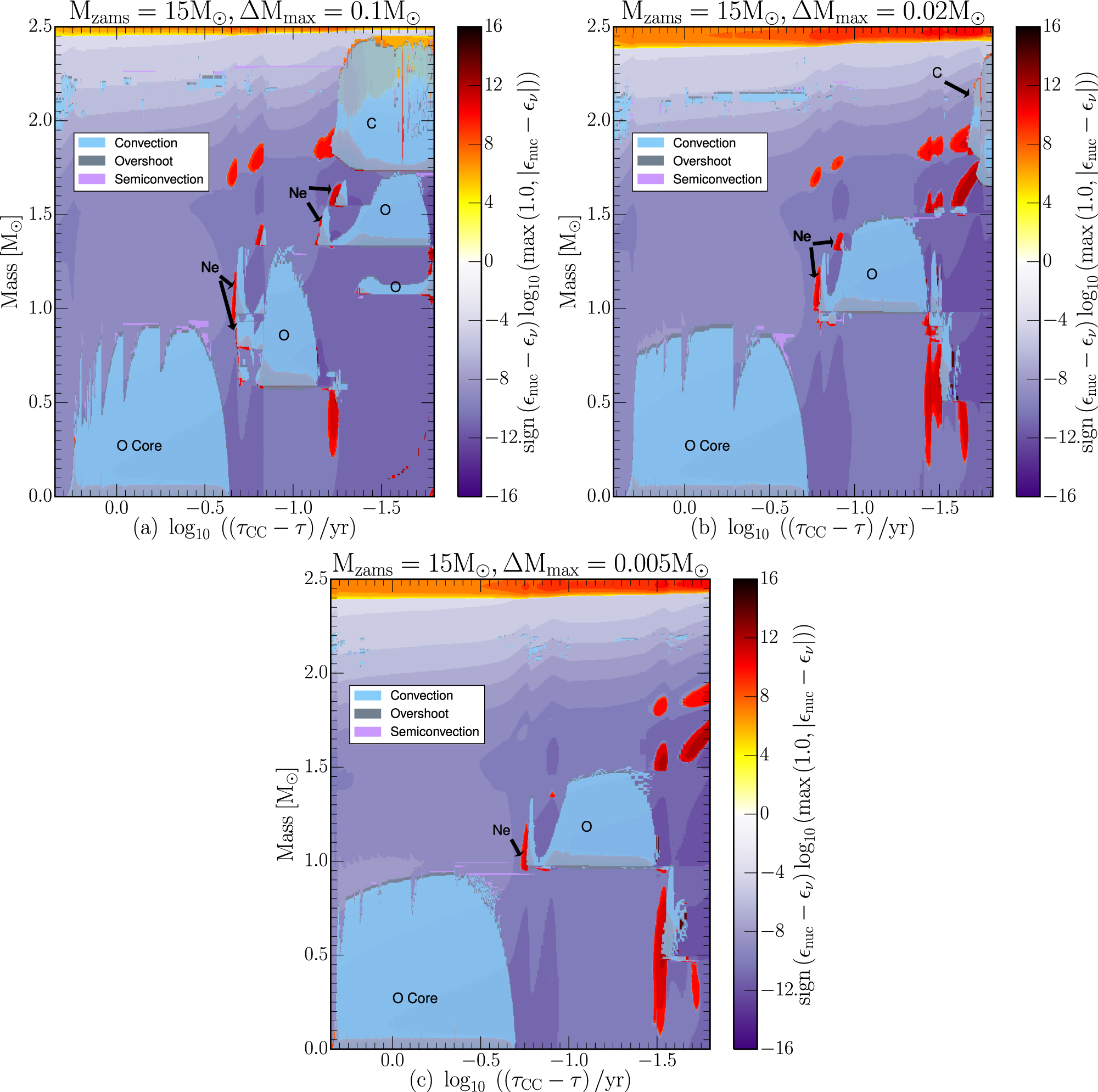
Figure 25. Stable isotopes from hydrogen to zinc for the  , 20, 25, and 30
  models with mass-loss,
 , and the mesa_204.net reaction network. The x-axis is the atomic mass number. The y-axis is the logarithmic ratio of the model mass fraction to the Grevesse & Sauval (1998) solar mass fraction. The most abundant isotope of a given element is marked by an asterisk, and isotopes of the same element are connected by solid lines.
Download figure:
Standard image High-resolution image
Isotopes in Figure 25 heavier that about calcium will be strongly impacted by the explosion. Up to calcium, however, it generally makes little difference whether the pre-SN or the exploded yields are used (e.g., Timmes et al. 1995). In a forthcoming effort we anticipate exploding the pre-SN models examined in this paper. With this limitation of interpreting pre-SN yields in mind, the overall average production factor of  for the
 model and rising to
  for the
 model are commensurate with existing pre-SN yields (e.g., Woosley & Weaver 1995; Limongi & Chieffi 2003; Chieffi & Limongi 2013) and the production factors needed by galactic chemical evolution models (e.g., Gibson et al. 2003) to reproduce the solar composition. Part of the spread below calcium is a consequence of uncertain physics in the MESA models: the treatment of convective, semiconvective, and overshoot mixing, the parameterization of mass-loss, nuclear reaction rates, and residual uncertainty in the measured solar abundances. Post-SN, the yields for isotopes with
  will also sensitively depend on the choice of explosion dynamics (Paxton et al. 2015).
The light isotopes  Li, 9Be, and
  are not plotted in Figure 25 as the primary source of these isotopes is commonly taken to be Big-Bang nucleosynthesis (e.g., Coc et al. 2012; Cyburt et al. 2016), spallation of CNO nuclei in the interstellar medium by cosmic rays (e.g., Reeves et al. 1970; Olive & Schramm 1992; Fields et al. 2000; Ramaty et al. 2000; Prantzos 2012), or the ν-process during the explosion (e.g., Woosley et al. 1990; Balasi et al. 2015).
The isotopes  and 14N are underproduced in Figure 25 by
  relative to the average overproduction factor for the
 model and by
  relative to the average overproduction factor for the
 model. This is consistent with the bulk of these isotopes being produced during CNO processing and dredged-up material from helium-shell flashes in intermediate- and low-mass stars (Iben & Truran 1978; Renzini & Voli 1981; Doherty et al. 2014; Karakas & Lugaro 2016).
The solar 29Si abundance is  times larger than the solar 30Si abundance, in concordance with observations of some individual stars (Peng et al. 2013) and pre-solar silicon-carbide grains (e.g., Hoppe et al. 2010), but it disagrees with common models of 1D core-collapse supernova, SNe Ia, and AGB stars (e.g., Timmes & Clayton 1996; Lugaro et al. 1999; Lewis et al. 2013; Wasserburg et al. 2015). It is curious that the 30Si abundance, normalized to solar in Figure 25, is larger than the 29Si abundance in the
  and 30
  models, but traditionally smaller in the
  and 25
  models.
The isotope 40K has the largest production factor in the  and 30
  models of Figure 25. This isotope is also a special case as it is radioactive, but the half-life is long enough (1.248 × 10⁹ yr, Malonda & Carles 2002; Kossert & Günther 2004) that it is included in compilations of the solar composition. The overproduction factor may reflect an uncertain solar abundance.
4. SUMMARY AND DISCUSSION
We have investigated the range of variation in properties of MESA pre-SN models with respect to changes in spatial resolution, number of isotopes in the nuclear reaction network, and the inclusion of mass-loss. To make this assessment, we evolved 200 solar metallicity, nonrotating, single-star models of initial mass  = 15, 20, 25, and 30
  from the pre-MS to the onset of core collapse.
We found that the choice of spatial resolution can have a larger impact on the final states of these models, predominately by altering the state of the star during the MS. This small effect can then be compounded by the relative length of the MS, compared with later evolution stages, to have large impacts on the stellar structure. The choice of nuclear network is also found not to be insignificant even during core helium burning where larger nuclear networks can suppress CBPs. The combination of these effects compounds over the stellar evolution, leading to sometimes radically different behaviors between models with the same mass, including differences in the type of carbon and neon burning, behavior of C, Ne, and O shells during silicon burning, and in the final mass of the iron core. In the remainder of this section, we discuss our findings and compare them with previous efforts.
Hirschi et al. (2004) considered the pre-SN evolution of nonrotating solar metallicity stellar models with 
 from the ZAMS to core Si depletion. We compare the median values of He
 for our mass-loss models with
  , 20, and 25
  to their reported He-core mass values and find agreement of ≈
 . Additionally, we compare the median values of
  to their quantity,
  which denotes the mass coordinate where the main fuel for CO burning (4He) drops below 10−2. Our mass-loss models with
  = 15, 20, and 25
  agree to
  of their values.
The effect of nuclear and stellar input physics on pre-SN nucleosynthesis was considered by Rauscher et al. (2002). Their set of models was evolved using the 1D implicit hydrodynamics code KEPLER (Weaver et al. 1978; Woosley & Weaver 1988; Heger et al. 2000), using a small nuclear network to generate the energy (similar to our approx22.net) with a larger adaptive network for the nucleosynthesis following  nuclei from the MS to explosion. Overall, our median final Fe-core mass at core collapse agrees to within
  of their values. The largest difference is found when comparing the
 model. This, however, is not surprising and is stated in their investigation as possibly being a consequence of the merging of the O-, Ne-, and C-shells
  day before collapse. We find considerable variation in the behavior of the O-, Ne-, and C-shells with the choice of whether they merge dependent on the resolution and network chosen. For instance, in our 25
  and 30
  models, the C shell appears to "merge" or dissolve before collapse. There is a large difference in the input physics of their models worthy of mention: the mass-loss efficiency, convection parameterization, convective overshoot, and other mixing terms. On average, their 20
  and 25
  models lose
 more than our models.
Limongi et al. (2000) studied 13, 15, 20, and 25  solar metallicity models with the FRANEC code (Chieffi et al. 1998) up to iron-core collapse. In comparisons with their final state models, they find
  for their
 models; the 15
  models match our results, while their 20 and 25
  models have slightly lower
  values, but within our upper and lower bounds on
  . They do not appear to have the ICZ we see in our models as they suppress overshoot and use the Schwarzschild criterion. They also artificially suppress the formation of CBP during core helium burning. Comparing the locations of the shell masses, our models in general predict shell locations to be
 greater than those of Limongi et al. (2000). This may be due to differences in the choice of mixing parameters as well as the differences in behavior of the ICZ and SCZ between our models.
Sukhbold & Woosley (2014) studied the compactness of pre-SN cores in stars between 
 with KEPLER. Comparing the compactness parameter with their S-series models (nonrotating, solar metallicity, with mass-loss), we have good agreement for the 15, 20, and 25
  models for the compactness parameter measured when v = 1000
  . However, for the 30
  models, our value of
  is much higher than their value of
  , although this value is consistent with the lower edge of the values we find. KEPLER models do not reach
  until
until 
 , although the authors point out that above
 uncertainties in mass-loss can affect the results.
El Eid et al. (2004) studied  and 30
  stars with mass-loss up to the end of central oxygen-burning using the code described in The et al. (2000). On average, comparing the core masses at the ignition of each fuel, we find our models to be 0.5
  heavier than those of El Eid et al. (2004). This can be explained, as they use the Schwarzschild criterion everywhere and only study using Ledoux for convective boundaries in a 25
  model. When they do use the Ledoux criteria (which we use everywhere), they find that their core masses grow by 0.8
  , which places them within the values we find. Comparing the timescale needed to burn each fuel for the 15
  and the 25
  models, we find our values to be commensurate with their values, except for the length of carbon burning. For the 25
  models without mass loss, we find
  , while they find
  . Differences may be due to the definition used. When we compare our results with their Figure 9, for the time over which carbon has vigorously ignited, they have carbon burning
  , but their burning is convective at the center, while we find carbon burning in the 25
  to be radiative, likely because of the lower core mass that results from using the Schwarzschild criteria.
One should bear in mind the limitations of our studies: our neglect of rotation and magnetic fields; ambiguous fidelity to the underlying 3D physics in the MESA 1D models: the treatment of convective (Trampedach et al. 2014), semiconvective (Moore & Garaud 2016), and overshoot (Kitiashvili et al. 2016) mixing; the parameterization of mass-loss (e.g., Šurlan et al. 2012; Madura et al. 2013); potentially underestimated contributions from iron in the opacity (Blancard et al. 2012; Colgan et al. 2016; Krief et al. 2016a, 2016b; Turck-Chièze et al. 2016); and unaccounted-for uncertainties in the nuclear reaction rates (e.g., Sallaska et al. 2013; Fields et al. 2016).
This project was supported by NASA under the Theoretical and Computational Astrophysics Networks (TCAN) grant NNX14AB53G, by NSF under the Software Infrastructure for Sustained Innovation (SI2) grant 1339600 and grant PHY-1430152 for the Physics Frontier Center "Joint Institute for Nuclear Astrophysics—Center for the Evolution of the Elements" (JINA-CEE). L.D. acknowledges financial support from "Agence Nationale de la Recherche" grant ANR-2011-Blanc-SIMI-5-007-01. C.E.F. acknowledges partial support from Michigan State University under the College of Natural Sciences Early Start Fellowship Program. F.X.T. acknowledges sabbatical support from the Simons Foundation. This work made use of the Arizona State University Research Computing resources Saguaro and Ocotillo.
Software: MESA (Paxton et al. 2011, 2013, 2015), Python python.org, matplotlib (Hunter 2007), NumPy (van der Walt et al. 2011).