


Abstract
Frequency analysis of pulsating stars can be performed via several algorithms. Still, each of these methods has its own specific flaws which advocates for the use of as many tools as possible. However, the lack of simple programs with straightforward interface impedes such a goal. pdm13 is a new software dedicated to spectral analysis based on the phase dispersion minimization technique. Its graphical environment, combined with complementary tools, such as auto-segmentation, makes it a simple and powerful mean for frequency extraction. In this paper, a detailed description of the mathematical algorithms is presented. Then, we introduce the options and interface of pdm13. Finally, we compare the results from different case study using pdm13 and other programs.
1 INTRODUCTION
As a fundamental tool to study the internal structure of stars, asteroseismology has proven to be particularly relevant. Still, progress is limited by the data accuracy and by inherent discontinuities of ground-based observations. The improvements of investigation methods are essential to overcome such obstacles, even if these issues tend to vanish with space missions such as CoRoT and Kepler.
Frequencies and mode identification constitute an important part of the main data of asteroseismology. They can be obtained by performing a projection of a discrete photometric signal on a trigonometric basis. There are two different approaches to frequency extraction: the parametric and the non-parametric method. The first one is the most commonly used and referred to as a Fourier-based analysis as one fits a harmonic model function to the data. The second does not assume an a priori model for the photometric function. Period04 (Lenz & Breger 2005) is an example of the available instrument for such purpose based on parametric method. Stellingwerf's phase dispersion minimization (PDM) technique (Stellingwerf 1978) is an alternative to Fourier transform algorithms for frequency extraction. As underlined by its author (Stellingwerf 2011), this non-parametric method outmatches existing ones for specific cases, urging for complementary investigation via different algorithms. Unfortunately, the lack of graphical interface and simplicity prevents a widespread usage of PDM.
In this paper, we present a new graphical interfaced program based on the PDM method, pdm13. This application also includes new features such as auto-segmentation, Gauss–Newton least-squares fitting and cyclostationary modulation detection together with the usual set of tools provided by such programs like phase, residuals or significance plots. The current 1.0 version and sources are available at forge.oca.eu/trac/PDM13.
2 THEORY AND METHOD
2.1 PDM
For frequency that is not present in the data, we will find ΘPDM ≈ 1.
2.2 Auto-segmentation
As underlined by Stellingwerf (2011), the computation time is greatly reduced when performing a first frequency search using a small segment rather than over the whole data sets. Besides, aliases due to gaps can also be diminished by such an approach. Nevertheless, the previous version of PDM relied on a threshold value defined by the user to determine if the time span between two points was a significant gap. The auto-segmentation algorithm is able to detect automatically each segment allowing a more simple and precise process.
For a given set of N data points ni(ti;mi), where ti and mi are the respective time and magnitude, the idea is to compute the delay between two following data points Δti = ti + 1 − ti and to detect any discontinuities using the Lee & Heghinian test (Lee & Heghinian 1977).
Therefore, we can estimate the probability that a discontinuity occurs at time τ. However, the Lee & Heghinian algorithm's computation time increases rapidly for rich data sets. Thus, we have implemented a recursive method reducing the complexity to |$\mathcal {O}(n)$|.
As this method broadens the spectral features from 1/T to 1/Tj, where T is the total time base and Tj the total time of the longest segment, we need to perform a second scan including gaps near the best candidate given by the first step.
2.3 Gauss–Newton algorithm
In former version of PDM, the amplitude associated to the best candidate frequency was the one of the mean curve. We have added a least-squares fitting algorithm which allows further investigation and comparison of the obtained value.
After a first scan, the residuals are calculated using the Stobie method (Stobie 1970). One can choose to remove only the extracted frequency from the signal or the signal mean curve.
2.4 Modulation detection and Blazhko effect
Based on this property, the program will divide the data in sub-segments and compute mean values for each of them. Then, the PDM algorithm will look for periodicity in the resulting file giving a best candidate for modulation frequency.
3 pdm13 INTERFACE
The graphical interface is divided in three parts.
Light curve module: within this module, the user can import, export, edit and plot the time string data.
PDM module: this module is dedicated to the extraction of frequencies – including multiple period and Blazhko modulation. As we have already mentioned, the PDM algorithm is used for this purpose. The user can also obtain a significance plot related to the extracted frequency – using the Beta function test or the Monte Carlo test.
Gauss–Newton module: in the third part, the Gauss–Newton algorithm performs a least-squares fit to obtain the amplitude and phase related to each selected frequency.
Besides, the Configuration menu allows more control on the automated parameters.
3.1 Light Curve tab
In this tab (Fig. 1), time series can be imported, exported, appended and edited. Furthermore, data points can be plotted using the Display Graph button.
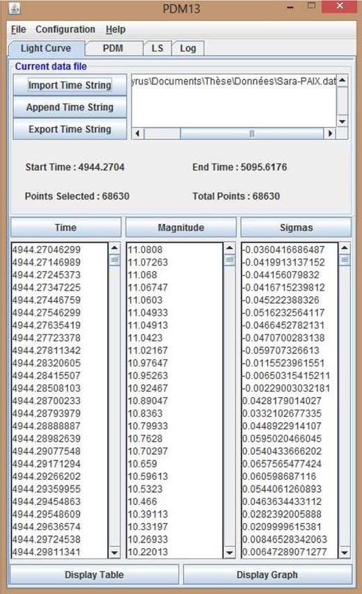
Light curve module.
Each plot can be manipulated using directly the mouse to zoom on a specific area or by choosing the Select ViewPort or View all in the Zoom menu. Likewise, each graph can be printed or exported in PNG/EPS format using the Graph menu.
3.2 PDM tab
This tab is divided into two parts: a panel which contains the available settings and a list box where PDM results are displayed (see Fig. 2).
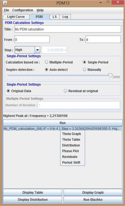
PDM module.
In the first part called PDM Calculation Settings, the frequency range and step can be edited as well as the title of the theta plot. The step between each investigated frequency is automatically fixed according to the given data. A Custom option is available to set this option manually.
The panel on the one hand permits to program numerous loops in order to look for multiple periods. The number of loops has to be specified in the Multiple-Period Settings block. On the other hand, it enables the user to set his own parameters for the segment detection or to let the program work on its own as already discussed. In manual mode, the program will look for gaps greater than a specified multiple – defined by segdev – of the average time between each of the data points. Using this mode is particularly interesting when a single segment is needed to avoid important bias due to small time coverage.
After the first run, the corresponding residuals are calculated. By switching the Single-Period Settings to Residual at original, the algorithm looks for a significant period in the pre-whitened data from the selected tab in the list box. Moreover, the user can choose to add the extracted frequency with a given number of harmonics to the LS tab after each calculation.
For each analysis, a line is added to the list box. This line contains the name and the parameters used for the calculation. Different options are available when right clicking on one of the tabs. First, the Theta Graph and Theta Table can be displayed. Equivalent to the Fourier spectrum, their minimum shows an a priori significant frequency. The pop-up menu also gives access to the Distribution Plot and table as well as the Period-Shift graph – if these options have been activated in the Configuration menu.
The residuals obtained after the selected analysis can also be plotted using this menu. Finally, the phase plot of the light curve at the best candidate frequency can be represented using the Phase plot option as well as the fit curve by selecting Fit Curve in the Curves menu.
At the bottom of the panel, different buttons give direct access to some of the plot and table already mentioned. The Run Blazhko button starts a direct scan for modulation frequency. The resulting file will have a ‘[Blazhko]’ prefix in the list box.
3.3 LS tab
Each frequency extracted, along with their harmonics, ends up in this part (Fig. 3). Frequencies, amplitudes and phases are imported or exported using the corresponding button. The Calculate button launches the least-squares fitting for all the selected items according to the formula specified in the upper panel. New frequencies can be added manually. Mathematical operations are accepted as long as they start with an = sign. For instance, in f2, the following line ‘ = 2*F1’ will be replaced by the double of the first frequency.
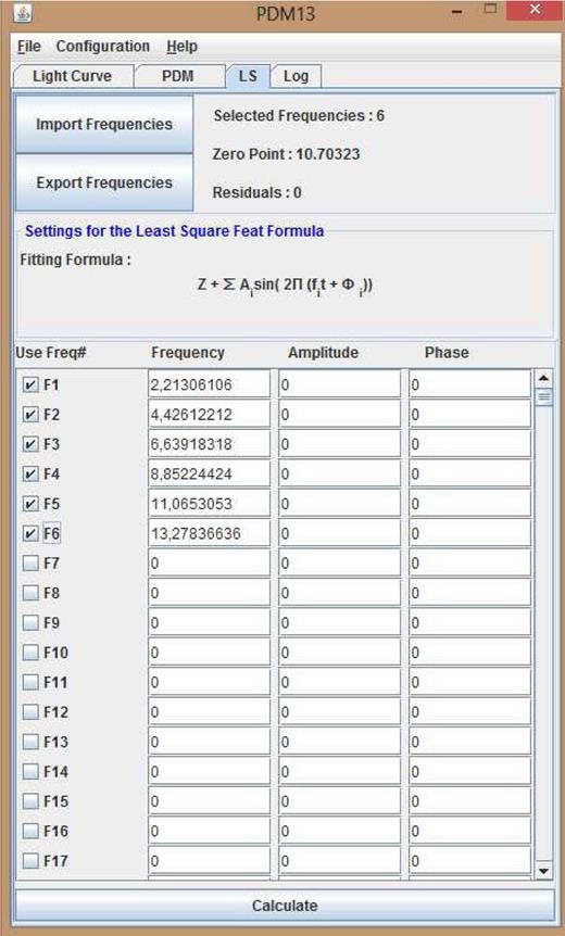
Gauss–Newton module.
Also, some information about the current fit are displayed such as Zero-Point, Selected Frequencies, Residuals.
3.4 Menu bar
Along with the usual possibilities found in a menu bar – save, load, new project, import, export – the Configuration menu allows the user to have more control on the PDM process (Fig. 4).

Option window.
The Set Bin Type offers three possibilities: 10/1, 5/2, auto. The auto option will let the program choose by itself which type of bin should be used. If the 10/1 option is selected, 10 or a 100 bins will be used – depending on the number of data points – to cover a period with no overlap between each of the data points. The 5/2 option is similar except that there is a half coverage between each of the bins which is more convenient for data sets with less than 100 points and produces less noise.
The Set Fit Type can be set to Linear Fit or Spline Fit. The latter gives a smoother fit of the bin means.
4 CASE STUDY AND DISCUSSION
Stellingwerf presented two case studies of artificial data strings where the PDM algorithm outperforms the Lomb–Scargle technique (Stellingwerf 2011). We carry on this study by showing the effect of accurate segmentation on the outcome of the computation.
The first one is a series of narrow pulses with unevenly distributed gaps (Fig. 5). The following curves correspond, respectively, to the frequency analysis for a Fourier-type method, PDM with no segmentation, PDM with manual segmentation and pdm13 with auto-segmentation. The details of the auto-segmentation are shown in Table 1. It is clear, as already stated, that PDM curve is more precise with narrower spectral lines and less prominent side lobes. What is even more noticeable is that aliases are smaller when considering the auto-segmentation result.
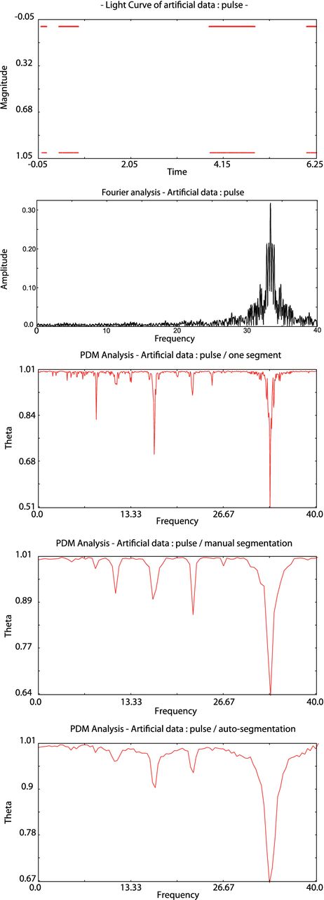
From top to bottom: Artificial data of several narrow pulses periodically spaced (T = 0.03 d) with unevenly distributed gaps; Fourier spectrum; pdm13 plot with no segmentation; pdm13 plot with manual segmentation; pdm13 plot with auto-segmentation.
Auto-segmentation of artificial data: pulse.
| Segment number | Start point | Number of points | Tstart | Trange |
|---|---|---|---|---|
| 1 | 0 | 126 | 0.001 | 0.125 |
| 2 | 126 | 440 | 0.407 | 0.439 |
| 3 | 566 | 1033 | 3.811 | 1.032 |
| 4 | 1599 | 221 | 6.019 | 0.22 |
| Segment number | Start point | Number of points | Tstart | Trange |
|---|---|---|---|---|
| 1 | 0 | 126 | 0.001 | 0.125 |
| 2 | 126 | 440 | 0.407 | 0.439 |
| 3 | 566 | 1033 | 3.811 | 1.032 |
| 4 | 1599 | 221 | 6.019 | 0.22 |
The second example was originally meant to show flaws in the Lomb–Scargle results in the case of a complex signal while PDM managed to obtain the accurate main frequency. We will push further this example by showing that adding gap in such case may lead to similar imprecise value unless the auto-segmentation option is used. The curve is shown in Fig. 6 along with the corresponding Fourier and pdm13 spectrum, without and with the auto-segmentation option. The results of the segment auto-detection are available in Table 2. As indicated, the manual segmentation and the Lomb–Scargle show an erroneous main period of 1 per day. Such an issue can be overcome by not performing segmentation but this will increase the calculation time.
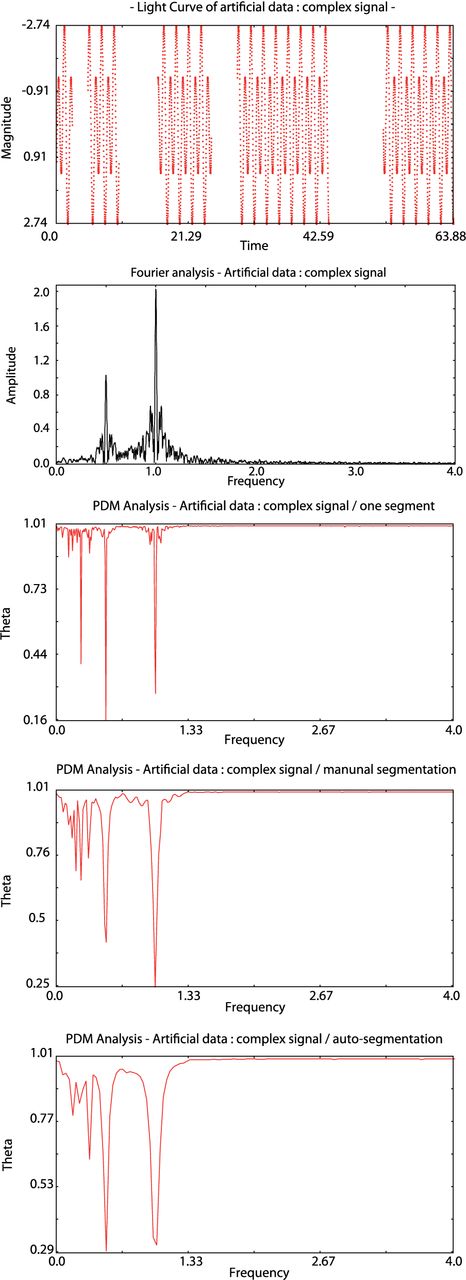
From top to bottom: Artificial data of complex signal made of two sinusoids (T1 = 1 d and |$T_2 = \frac{1}{2}\; {\rm d}$|) with unevenly distributed gaps; Fourier spectrum; pdm13 plot with no segmentation; pdm13 plot with manual segmentation; pdm13 plot with auto-segmentation.
Auto-segmentation of artificial data: complex signal.
| Segment number | Start point | Number of points | Tstart | Trange |
|---|---|---|---|---|
| 1 | 0 | 251 | 0 | 2.5 |
| 2 | 251 | 501 | 5 | 5 |
| 3 | 752 | 864 | 16.27 | 8.63 |
| 4 | 1616 | 1480 | 29.04 | 14.79 |
| 5 | 3096 | 1135 | 52.54 | 11.34 |
| Segment number | Start point | Number of points | Tstart | Trange |
|---|---|---|---|---|
| 1 | 0 | 251 | 0 | 2.5 |
| 2 | 251 | 501 | 5 | 5 |
| 3 | 752 | 864 | 16.27 | 8.63 |
| 4 | 1616 | 1480 | 29.04 | 14.79 |
| 5 | 3096 | 1135 | 52.54 | 11.34 |
Our last test cases are the Blazhko RR Lyrae star S Arae (|$\alpha = 17^{\rm h}59^{\rm m}10 {.\!\!^{\rm s}}73$|, δ = −49°26′00|${^{\prime\prime}_{.}}$|45, J2000; Chadid et al. 2010) observed from Antarctica using the Photometer AntarctIca eXtinction (PAIX) telescope and the eclipsing binary star 000202−6653.3 (|$\alpha = 0^{\rm h}02^{\rm m}02 {.\!\!^{\rm s}}0$|, δ = −66°53′17|${^{\prime\prime}_{.}}$|9, J2000 with Vmax = 12.16 mag) from the ASAS Catalogue (Pojmanski 2002). These case studies focuses on pdm13 auto-segmentation ability (Tables 3 and 4). Even with a very high duty cycle for a ground-based observation site, S Arae light curve shows numerous gaps (Fig. 7). Running the algorithm using manual segmentation and a segdev value of about 500 leads to irrelevant results such as f1 = 1.1065 d− 1 ± 3.303 662E − 4 or f1 = 0.4426 d− 1 ± 3.303 662E − 4 showing the importance of this parameter in the PDM analysis. By performing an accurate and automated segmentation with the auto-segmentation option, we avoid such obstacle. Indeed, the algorithm was able to isolate 23 clusters ending up with f1 = 2.2129 d− 1 ± 3.303 662E − 4 (Fig. 8) as obtained by Chadid et al. with Period04. The Blazhko behaviour is clear in the phase plot folded with the main frequency (Fig. 9). The investigation for a modulation frequency leads to a value of fm = 0.1999 ± 3.303 662E − 4. Similarly, running pdm13 on 000202−6653.3 (Fig. 10) using one segment ends up with a main frequency f1 = 3.562 051 683 d− 1 ± 2.537 101E − 5 while the correct period of 3.062 081 498 d− 1 ± 2.537 101E − 5 is obtained using the auto-segmentation option (Figs 11 and 12).
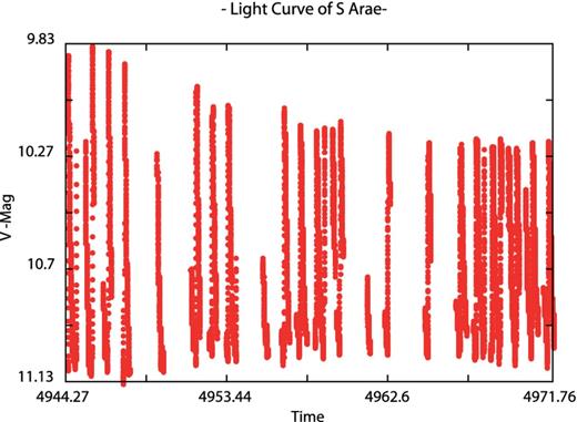
PAIX light curve of S Arae.
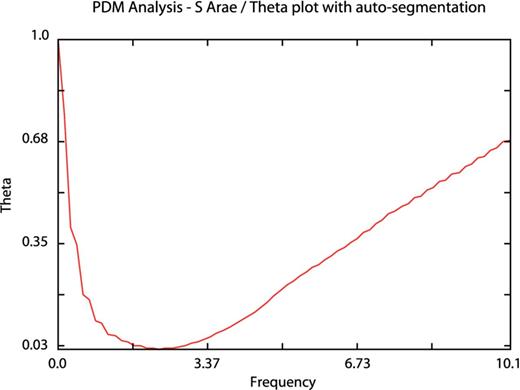
Theta plot of S Arae using auto-segmentation.
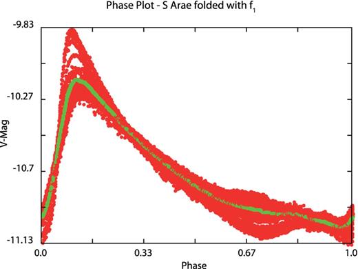
Folded PAIX light curve with main pulsation P1 (in red) and mean curve (in green).
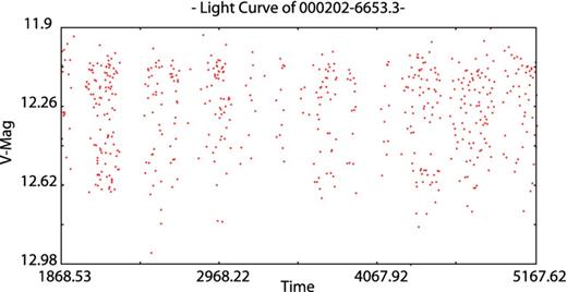
Light curve of 000202−6653.3.
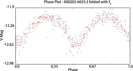
Folded 000202−6653.3 light curve with main pulsation P1.
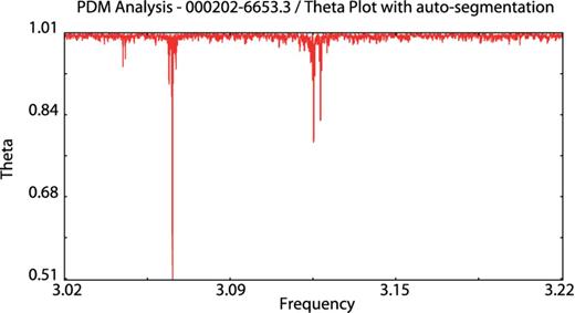
Theta plot of 000202−6653.3 using auto-segmentation.
Auto-segmentation of S Arae data.
| Segment | Number of | Tstart | Trange | |
|---|---|---|---|---|
| number | Start point | points | ||
| 1 | 0 | 525 | 4944.270 463 | 0.478 773 |
| 2 | 525 | 510 | 4945.264 85 | 0.486 643 |
| 3 | 1035 | 501 | 4946.283 692 | 0.466 146 |
| 4 | 1536 | 375 | 4947.396 019 | 0.363 356 |
| 5 | 1911 | 357 | 4949.333 16 | 0.340 74 |
| 6 | 2268 | 548 | 4951.238 519 | 0.522 152 |
| 7 | 2816 | 480 | 4952.233 16 | 0.451 782 |
| 8 | 3296 | 573 | 4953.223 125 | 0.553 935 |
| 9 | 3869 | 267 | 4955.306 25 | 0.256 285 |
| 10 | 4136 | 492 | 4956.313 623 | 0.466 666 |
| 11 | 4628 | 711 | 4957.198 09 | 0.589 966 |
| 12 | 5339 | 678 | 4958.208 241 | 0.585 671 |
| 13 | 6017 | 294 | 4959.203 38 | 0.165 532 |
| 14 | 6311 | 391 | 4959.440 66 | 0.373 692 |
| 15 | 6702 | 174 | 4961.188 785 | 0.158 981 |
| 16 | 6876 | 405 | 4962.178 079 | 0.286 84 |
| 17 | 7281 | 468 | 4964.443 495 | 0.346 366 |
| 18 | 7749 | 681 | 4966.213 634 | 0.562 13 |
| 19 | 8430 | 860 | 4967.196 979 | 0.612 361 |
| 20 | 9290 | 907 | 4968.155 139 | 0.644 363 |
| 21 | 10 197 | 900 | 4969.150 035 | 0.638 946 |
| 22 | 11 097 | 987 | 4970.134 78 | 0.702 176 |
| 23 | 12 084 | 861 | 4971.1496 41 | 0.614 896 |
Auto-segmentation of 000202−6653.3.
| Segment | Start point | Number of | Tstart | Trange |
|---|---|---|---|---|
| number | points | |||
| 1 | 0 | 19 | 1868.525 78 | 80.990 11 |
| 2 | 19 | 105 | 2033.890 15 | 237.643 88 |
| 3 | 124 | 38 | 2439.899 22 | 124.752 79 |
| 4 | 162 | 24 | 2620.545 11 | 60.973 82 |
| 5 | 186 | 2 | 2744.919 71 | 14.003 48 |
| 6 | 188 | 58 | 2818.923 83 | 225.600 01 |
| 7 | 246 | 2 | 3107.919 24 | 8.002 65 |
| 8 | 248 | 9 | 3146.915 75 | 65.000 62 |
| 9 | 257 | 1 | 3276.728 05 | 0 |
| 10 | 258 | 2 | 3356.578 37 | 3.0075 |
| 11 | 260 | 10 | 3382.574 44 | 32.940 71 |
| 12 | 270 | 4 | 3526.901 36 | 28.008 03 |
| 13 | 274 | 1 | 3584.860 65 | 0 |
| 14 | 275 | 20 | 3615.824 22 | 61.895 43 |
| 15 | 295 | 24 | 3700.5908 | 75.930 75 |
| 16 | 319 | 15 | 3849.922 97 | 63.015 05 |
| 17 | 334 | 12 | 4084.586 56 | 55.936 76 |
| 18 | 346 | 80 | 4228.930 63 | 269.614 14 |
| 19 | 426 | 93 | 4564.919 18 | 307.606 38 |
| 20 | 519 | 51 | 4933.9213 | 233.700 66 |
5 CONCLUSION
The different examples presented in this paper show that a spectral analysis based solely on the Fourier-type method can lead to incorrect conclusions. Such assessment advocates for complimentary frequency extraction tools. To achieve such a goal, these tools need to be simple and powerful to allow a widespread use. pdm13 reaches this aim by combining a graphical interface with automated processes. We have showed how these can outperform existing software on specific cases.
One of the main feature, the auto-segmentation based on the Lee & Heghinian's technique, is originally intended to detect one major change in the data sets. Still our recursive approach, which was first meant to reduce computation time, permits to detect multiple discontinuities. Consequently, we were able to obtain an accurate segmentation greatly reducing aliases and enhancing the result curve.
