


Abstract
We report on the testing of the centrosymmetry parameter (CSP), an indicator of deviation from centrosymmetry of a source brightness distribution. This indicator is derived from the spectral distribution of the triple product measured over three baselines of an optical interferometer. Numerical simulations using parametric toy-models (separated or transiting binary, one-spot model), generated with the spidast software, are applied to the VLTI /AMBER facility in the K band (2.2 μm). The simulations show that, in case of centrosymmetry, the CSP parameter is in agreement with the usual phase of the spectral mean of the triple product (called GCP, global closure phase). To justify the preferential use of CSP rather than GCP, we show situations with asymmetric geometries for which GCP diagnoses centrosymmetry, while CSP does not. Using realistic Roche lobe-filling binary and hydrodynamic convective models, we show that CSP can also be used as an indicator for geometric similarity between physical and toy-models. Thus, dealing with real data, the toy-model parameters can be fitted on the measured CSP values, in order to assess the input-parameter values of the most suitable complex physical model that will be used to interpret the data.
1 INTRODUCTION
With the advent of interferometry, most celestial sources can no longer be considered as point sources. Instead, asymmetries in their light distribution appear at various spatial scales. Let us mention the following astrophysical environments where deviations from centrosymmetry occur in the brightness distribution (e.g. Berger et al. 2012).
most of stars (more than 50 per cent in the solar neighbourhood) form in binary or multiple systems, due to fragmentation of protostellar molecular clouds;
most planetary nebulae (more than 80 per cent) are non-spherical, because of binarity, stellar winds, and magnetic fields;
circumstellar dust shells produced by mass-loss show a clumpy distribution; accretion discs in binary systems are twisted or warped;
stellar activity and convection produce inhomogeneous stellar surface structures, with spots, faculae, granules, and supergranules.
If not based on direct imaging, the detection of surface brightness asymmetries (SBAs) usually relies on the so-called triple product, involving complex visibilities from interferometric observations using three simultaneous apertures. To measure SBA with a single indicator, Ragland et al. (2006) and Tatebe et al. (2006) used the triple product to define the so-called global closure phase (GCP; it is called ‘global’ because it involves integrals over the spectral band [λmin, λmax]). The use of this kind of global indicator is essential if we want to search for asymmetries through archive data dealing with sample of objects observed with limited uv-coverage, thus allowing no reliable image reconstruction.
When searching for SBA at the surface of asymptotic giant branch (AGB) stars, Cruzalèbes et al. (2013a) (Paper I; their table 3 and fig. 14) showed that the GCP parameter sometimes leads to ‘false negatives’, i.e. values close to zero (as usual for centrosymmetric distributions) despite indications that the star exhibits SBAs (see the values obtained for TX Psc and W Ori). To avoid such false negatives, a more robust parameter has been introduced in Paper I, the so-called centrosymmetry parameter (CSP) dedicated to the detection of source brightness asymmetries using spectro-interferometric data (in the present case, VLTI/AMBER data in the K band at 2.2 μm).
The aim of this paper is to show how CSP behaves on well-controlled situations depicted by simple models like binary systems or stellar surfaces covered by a single (dark or bright) spot, before applying this parameter to diagnose SBA on AGB stars in a forthcoming paper. Our present study will thus confront CSP with GCP in such simple situations, and at the same time, show how one-spot models differ from binary models when probed by such parameters. In both situations (binary stars and spots), CSP and GCP have been computed for more realistic models as well, namely a tidally deformed Roche lobe filling star (generated following the method described in Siopis & Sadowski 2012 and in Paladini et al. 2014) including limb- and gravity-darkening, and a hydrodynamical model of the surface convection of a red supergiant (RSG) star (Freytag et al. 2012). Moreover, we investigate the properties of the simple (geometric toy) models approximating these realistic models as judged from the similar values for their CSP (or GCP) parameters. We stress for instance that a tidally deformed star (the only visible component of a binary system) may be represented by a one-spot model with the spot located close to the limb of the star. Thus, when a simple-model fit to spectro-interferometric data leads to such a situation, it hints at the presence of a tidally deformed star.
The paper is organized as follows. In Section 2, we recall the definition of the triple product. In Section 3, we present the motivation for using CSP and the way this indicator has been built. In Section 4, we present the morphological toy-models used to show, on simulated data, the ability of CSP to measure asymmetries that are not detected by GCP. In Section 6, we present CSP values obtained on a Roche lobe-filling binary model. In Section 7, we present CSP values obtained with a hydrodynamic convective model. In Section 8, are given concluding comments on the potential of using CSP in various contexts, that will be the subject of a forthcoming paper.
The results and graphical outputs presented in the paper have been obtained using the modular software suite spidast,1 created to calibrate spectro-interferometric measurements, particularly those obtained with VLTI/AMBER, and to interpret them by using chromatic models (Cruzalèbes, Spang & Sacuto 2008; Cruzalèbes et al. 2010, 2013b). The simulations are done for the VLTI sub-array (VISA) configuration, with the AMBER medium-resolution spectral mode in the K band (MR–K): spectral resolution R = 1500; central wavelength λc = 2.3 μm; and full wavelength range [2.126 μm–2.474 μm].
2 THE NEED FOR THE TRIPLE PRODUCT
2.1 The visibility function
The Fourier Transform of a centrosymmetric brightness distribution is real, i.e. has a null imaginary part. In practice, atmospheric turbulence adds random phase shifts αi-αj to the phase of the measured visibilities at the frequency |$\boldsymbol {f_{ij}}$|, so that the measured visibility Vij is multiplied by the phasor exp (i(αi − αj)). Thus, centrosymmetric objects observed through the terrestrial atmosphere show complex Fourier spectra, with non-null imaginary parts.
2.2 The triple product
If the centrosymmetric source is off-axis, the phase of its Fourier spectrum φ varies linearly with the spatial frequency, so that |${\varphi (\boldsymbol {f_{13}})=\varphi (\boldsymbol {f_{12}})+\varphi (\boldsymbol {f_{23}})}$| and, subsequently, also here the imaginary part of |$\scr {T}_{123}$| (denoted ℑ123) is equal to zero. Let us mention that if the source is unresolved (whatever its intrinsic morphology), we also find ℑ123 = 0, since V is equal to unity, at all spatial frequencies. To avoid this ambiguity, we consider, in our study, only stellar objects with resolved diameters. Thus, with our targets, a non-zero value of ℑ123 is an unambiguous indication that the object brightness distribution deviates from centrosymmetry.
3 INDICATORS FOR DEPARTURE FROM CENTROSYMMETRY
3.1 The usual indicator: the global closure phase (GCP)
The visibilities are measured over a finite spectral band, thus leading to a unique value of GCP. When this value significantly departs from zero degree (taking into account the uncertainty), the degree of asymmetry of the brightness distribution is measured (over the considered aperture triplet), otherwise centrosymmetry is the resulting conclusion. Note that information from possible variation over the spectral band is then ignored.
3.2 The use of the spectral information
Our data (visibilities) are obtained point-wise over the observed spectral band, with a large number of individual spectral channels (more than 500 with AMBER MR–K). This situation invites to explore the spectral behaviour of GCP, resulting in as many GCP values as the number of spectral channels. This enables to track possible morphological variations especially when spectral lines are present in the observed spectral band (as it is frequently the case with cool stars).
To get a single indicator for asymmetry, a first possible approach is to integrate over the spectral band the monochromatic closure phases computed from monochromatic triple products. But this approach might result in a completely false indication of asymmetry even with centrosymmetric brightness distributions (e.g. when a π-shift of the closure phase occurs within the observed spectral band, caused by the zero-crossing of the visibility function).
A second possible approach is to use the imaginary part of monochromatic triple products. While working on real data (Paper I), it appeared in some cases that the imaginary part was not remaining close to zero over the whole spectral band, but presented a slope (see e.g., TX Psc and W Ori in fig. 13 of Paper I). This indicates that the brightness distribution truly deviates from centrosymmetry. However, the conclusion obtained by using GCP was ‘centrosymmetry’ (see again the position of TX Psc and W Ori in fig. 14 of Paper I).
In the remainder of the paper, we call ‘false negatives’ these specific situations of missed asymmetry detection.
3.3 The centrosymmetry parameter (CSP)
Even though the definitions of CSP and GCP look similar, there is no algebraic expression linking them, unless one adopts the (unrealistic) hypothesis that ℑ123 and ℜ123 are wavelength-independent. In that case, one would have CSP = |Φcl|, where Φcl is defined in equation (3).
At this point, the extra diagnosis power offered by CSP over GCP may not be very apparent, since both quantities are based on the imaginary part of the triple product. To demonstrate the advantage of CSP, we used toy-models with known asymmetries and evaluated the corresponding CSP and GCP values. This is done in Section 4.1 for the binary model, and in Section 4.2 for the one-spot model.
4 COMPUTING CHROMATIC MODELS
4.1 The binary model
Let us consider the binary model, containing a central primary source of diameter ϕ1, and a shifted secondary source of diameter ϕ2, located at the angular distance ε2 from the primary, with a position angle (PA) θ2. The diagram at left of Fig. 1 shows the general geometry used to compute the polar Fourier Transform for the binary model. The points C1 and C2 are the centres of the primary and secondary components, respectively, θ2 being the PA of C2. The small disc contained in the disc of the primary source represents the secondary source. Its Fourier Transform is computed by the integration of the polar coordinates r and θ, respectively, when moving the point M radially from P− to P+, along the directions lying between the limiting angles θ− and θ+, given by the tangential points P0 − and P0 +. Thus, our composite source comprises three components: the primary disc (index 1), the secondary (index 2) shifted by an amount ε2, and the part of the primary disc occulted by the secondary (index 1–2) shifted by the same amount.
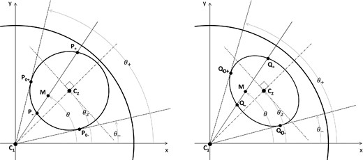
General geometry used for each model. Left-hand diagram: binary model (eclipse situation); right-hand diagram: one-spot model.
For the simulations shown in the present study with composite models, we consider the primary source as a limb-darkened disc of outer angular diameter ϕ1 and temperature T1, and the secondary as a uniform-disc blackbody of diameter ϕ2 and temperature T2.
- For θ, the limiting directions are tangent to the circle, hence immediatelyIf the secondary source masks the centre of the primary disc, i.e. for ε2 ≤ ϕ2/2, we use θ± = θ2 ± π/2.(15)\begin{eqnarray} \theta _{\pm } = \theta _{2} \pm \arcsin \left(\frac{\phi _{2}}{2\varepsilon _{2}}\right). \end{eqnarray}
- For r, the distance between the running point M and the centre C2 must be less than or equal to the radius ϕ2/2 which gives (using Pythagora's theorem)(16)\begin{eqnarray} \left(r \cos \theta - \varepsilon _{2} \cos \theta _{2} \right)^2+\left(r \sin \theta - \varepsilon _{2} \sin \theta _{2} \right)^2 \le \left(\frac{\phi _{2}}{2}\right)^{2}. \end{eqnarray}
Fig. 2 shows the (u, v)-distribution of the modulus of the visibility (λ = 2.19 μm) for the single uniform disc with 6 -mas diameter (left-hand panel), and the binary model (right-hand panel), with parameters given in Table 1 (secondary-to-primary flux ratio equal to 1:36).

Distribution of the modulus of the visibility in the (u, v)-plane. Left-hand panel: single-disc model. Right-hand panel: binary model.
Fiducial parameters of the binary and the one-spot models.
| Model | T1 | ϕ1 | T2 | ϕ2 | ε2 | θ2 |
|---|---|---|---|---|---|---|
| (K) | (mas) | (K) | (mas) | (mas) | (deg) | |
| Binary | 4000 | 6.0 | 4000 | 1.0 | 18 | 71 |
| one-spot | 3650 | 6.3 | 4000 | 3.0 | 1.9 | 71 |
| Model | T1 | ϕ1 | T2 | ϕ2 | ε2 | θ2 |
|---|---|---|---|---|---|---|
| (K) | (mas) | (K) | (mas) | (mas) | (deg) | |
| Binary | 4000 | 6.0 | 4000 | 1.0 | 18 | 71 |
| one-spot | 3650 | 6.3 | 4000 | 3.0 | 1.9 | 71 |
The binarity causes oscillations in the modulus of the visibility, as it is shown in the right-hand panel of Fig. 2. The amplitude of oscillation increases with the secondary-to-primary flux ratio, and the frequency of oscillation (in the (u, v)-plane) increases with the primary to secondary distance.
Figs 3 and 4 present four panels (each containing four sub-panels), and are organized as follows. On the left-hand side of these figures (labels (a) and (c)) is shown what pertains to the linear configuration (A0–D0–H0), while on the right-hand side (labels (b) and (d)) is shown what pertains to the triangular configuration (A0–D2–H0). This latter case will be examined later on in Section 5. In both Figs 3 and 4, the top-panels (labels (a) and (b)) pertain to the binary model while the bottom panels (labels (c) and (d)) pertain to the one-spot model.
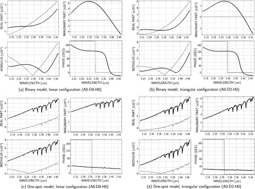
Spectral distributions of the triple product obtained with the linear A0–D0–H0 (left-hand panels) and triangular A0–D2–H0 (right-hand panels) array configurations, for the binary model (top); for the one-spot model (bottom). Thick lines: composite model (central star + secondary component or spot); thin lines: single central component model. Top left sub-panels: real part of the triple product. Top right sub-panels: imaginary part. Bottom left sub-panels: modulus. Bottom right sub-panels: phase of the triple product (in degree). For each panel, the associated GCP and CSP values are, respectively: 105° and 38° (a); 78° and 35° (b); 31° and 31° (c); 21° and 21° (d).

Variation of CSP (full thick line) and GCP (dashed thin line) obtained with the linear A0–D0–H0 (left-hand panels) and the triangular A0–D2–H0 (right-hand panels) configurations, versus the parameters of the binary model (top panels), and of the one-spot model (bottom panels).
Fig. 3 refers to the spectral distribution of the triple product, and in each panel are shown its real part, imaginary part, modulus and phase distributed in the four sub-panels. In addition, each diagram shows two traces: one for the binary model (thick line), the other for the single uniform disc (thin dashed line). For the binary model, the two components are aligned as parallel to the largest baseline (direction A0-H0, 71° from north, clockwise), thus giving the maximal spatial resolution.
To test the variation of CSP and GCP with the model parameters, we refer to what we call the fiducial values, given in Table 1 and used to produce Fig. 3.
Fig. 4 is dedicated to the behaviour of CSP and GCP versus several parameters of the models, and is organized similarly to Fig. 3, that is the panels on the left are for the linear configuration, and the panels on the right are for the triangular one. The panels at the top are for the binary model, and the panels at the bottom are for the one-spot model. In each sub-panel, the thick solid line is for CSP, and the thin dashed line is for GCP. For the panels at the top (binary model), the sub-panels refer to the following parameters: the diameter of the primary (top left), the diameter of the secondary (top right), the angular separation (bottom left), and the PA (bottom right). For the panels at the bottom (one-spot model), the sub-panels refer to the following parameters: the temperature of the spot (top left), the diameter of the spot (top right), the angular separation (bottom left), and the PA (bottom right).
We notice the large amplitude of variation of GCP, between −180° and 180°, caused by the use of the four-quadrant inverse tangent function (atan2 function), while CSP does not vary with so large an amplitude. In addition, CSP takes only strictly positive values. The curves show that specific values of the model parameters produce null GCP values (so leading to the erroneous conclusion of centrosymmetry):
one value of ϕ1 in the top left sub-panel,
two values of ϕ2 in the top right sub-panel,
four values of ε2 in the bottom left sub-panel, and
seven values of θ2 in the bottom right sub-panel,
while the other parameters are maintained at their fiducial values. These 14 sets of parameter values are gathered in the top part of Table 2, with the associated CSP values included in the last column (remember that GCP = 0° for any set of Table 2), the second part (bottom) being associated with the one-spot model (next section). A null GCP value means that the spectral distribution of the triple product shows an imaginary part with negative values compensating the positive values, and not that the model is centrosymmetric. Although we could think that finding a null GCP value associated with a non-null CSP value is an extreme and rare case, we must recall that, when dealing with real data which are subject to measurement errors, each GCP value smaller than its uncertainty can be incorrectly considered as indicator for centrosymmetry as well, as shown in table 3 of Paper I for the two targets TX Psc and W Ori, thus increasing the number of possible false detections of negative asymmetry.
Parameter sets of the binary model (top part) and of the one-spot model (bottom part), providing null GCP values with the linear configuration (A0–D0–H0). The last column gives the associated CSP values.
| ϕ1 | ϕ2 | ε2 | θ2 | CSP |
|---|---|---|---|---|
| (mas) | (mas) | (mas) | (deg) | (deg) |
| 6.00 | 1.00 | 18.00 | 161.0 | 0.0 |
| 6.00 | 1.00 | 18.00 | 14.8 | 18.5 |
| 6.00 | 1.00 | 18.00 | 36.4 | 20.7 |
| 6.00 | 1.00 | 18.00 | 105.6 | 20.7 |
| 6.00 | 1.00 | 18.00 | 127.3 | 18.5 |
| 6.00 | 1.00 | 18.00 | 145.3 | 5.2 |
| 6.00 | 1.00 | 18.00 | 176.7 | 5.2 |
| 6.00 | 1.00 | 4.87 | 71.0 | 5.2 |
| 6.00 | 1.00 | 10.00 | 71.0 | 18.5 |
| 6.00 | 1.00 | 14.81 | 71.0 | 20.7 |
| 6.00 | 1.00 | 19.78 | 71.0 | 21.5 |
| 6.00 | 5.98 | 18.00 | 71.0 | 59.4 |
| 6.00 | 8.02 | 18.00 | 71.0 | 28.0 |
| 1.27 | 1.00 | 18.00 | 71.0 | 31.4 |
| T2 | ϕ2 | ε2 | θ2 | CSP |
| (K) | (mas) | (mas) | (deg) | (deg) |
| 4000 | 3.00 | 2.63 | 71.0 | 4.1 |
| 9616 | 3.00 | 1.90 | 71.0 | 31.2 |
Parameter sets of the binary model (top part) and of the one-spot model (bottom part), providing null GCP values with the triangular configuration (A0–D2–H0). The last column gives the associated CSP values.
| ϕ1 | ϕ2 | ε2 | θ2 | CSP |
|---|---|---|---|---|
| (mas) | (mas) | (mas) | (deg) | (deg) |
| 1.63 | 1.00 | 18.00 | 71.0 | 14.7 |
| 6.00 | 1.00 | 18.00 | 13.7 | 9.5 |
| 6.00 | 1.00 | 18.00 | 36.7 | 17.4 |
| 6.00 | 1.00 | 18.00 | 104.8 | 18.1 |
| 6.00 | 1.00 | 18.00 | 127.9 | 8.6 |
| 6.00 | 1.00 | 18.00 | 145.0 | 6.8 |
| 6.00 | 1.00 | 18.00 | 160.4 | 6.9 |
| 6.00 | 1.00 | 18.00 | 177.9 | 11.4 |
| 6.00 | 1.00 | 4.82 | 71.0 | 2.1 |
| 6.00 | 1.00 | 10.24 | 71.0 | 17.1 |
| 6.00 | 1.00 | 14.89 | 71.0 | 17.9 |
| 6.00 | 1.00 | 19.89 | 71.0 | 17.5 |
| 6.00 | 6.06 | 18.00 | 71.0 | 42.3 |
| 6.00 | 6.66 | 18.00 | 71.0 | 22.7 |
| T2 | ϕ2 | ε2 | θ2 | CSP |
| (K) | (mas) | (mas) | (deg) | (deg) |
| 4000 | 3.00 | 2.55 | 71.0 | 3.2 |
| 9480 | 3.00 | 1.90 | 71.0 | 30.6 |
Let us also notice that the parameter set given in the first line of Table 2, obtained with θ2 = 161°, produces both a null GCP value and a null CSP one. The explanation of this result is straightforward: the orientation angle of the secondary has been chosen so that the orientation of the couple (161° = 71° + 90°, from north, clockwise) is perpendicular to the linear array (oriented 71° from north, clockwise). Here, the interferometer cannot detect the binarity (and any departure from centrosymmetry), since it has no spatial resolution along the direction of the couple.
4.2 The one-spot model
To generate synthetic spectro-interferometric data for the one-spot model, we use an approach to some extent similar to the one used for the binary model. Namely, we consider three discs as components: the central star (spectral radiance O1, diameter ϕ1), the spot (radiance O2, diameter ϕ2) shifted by the amount ε2 lying on the surface of the star, and the corresponding part of the star (same radiance as the star and same diameter as the spot) replaced by the spot. The expression of the composite Fourier spectrum is also given by equation (12), where |$\hat{O}_{1}$|, |$\hat{O}_{2}$|, and |$\hat{O}_{1-2}$| are the corresponding, respective, Fourier spectra of these components. Here again, the central source is assumed to be a limb-darkened disc of temperature T1.
For the spot, we assume it is a disc emitting radiation as a blackbody with temperature T2. This disc is seen as projected on to the plane perpendicular to the line of sight, and its apparent shape is roughly an ellipse, all the more flattened as the spot comes close to the stellar limb. Previous studies on RSGs demonstrated that spots may be modelled well by uniform ellipses (Young et al. 2000; Haubois et al. 2009; Baron et al. 2014). Fig. 1 shows the general geometry, in the ‘standard case’, used to compute the Fourier Transform of the composite brightness distribution. This standard case means that the shift is larger than half the minor axis of the ellipse (radial direction), and that the projected disc is not cut by the stellar limb. The complementary situation is considered separately later on. To take into account the shape of the projected spot, we use an elliptic shape whose minor axis is equal to μϕ2, where |${\mu =\sqrt{1-(2\varepsilon _{2}/\phi _{1})^{2}}}$| is the ratio minor to major axis, ε2 the angular distance between the centre of the stellar disc C1 and the centre of the ellipse C2. Actually the shape of the projected spot is not a perfect ellipse, but a faintly distorted one because the spot is lying on a sphere and not on a plane. However, including this small distortion in the computation would be rather meaningless for several reasons : (i) the one-spot model is in itself a coarse description of the brightness distribution and the weak distortion is not critical in this approach; (ii) the distortion is weak and is reasonably not likely to have a substantial effect on the result; (iii) the purpose of the modelled distribution is to examine the respective diagnosis from GCP and CSP, when working on identical geometries, and this goal is not corrupted by using such a weakly distorted elliptic shape.
Coming back to Fig. 3, dedicated to the spectral behaviour of the triple product, the bottom panels (labels (c) and (d)) refer to the one-spot model. We have on the left, the case of the linear configuration while the case of the triangular configuration is on the right. In each sub-panel are shown the real part (top left), the imaginary part (top right), the modulus (bottom left), and the phase in degrees (bottom right). Thick lines are for the one-spot model while thin lines are for the single disc only.
The stellar disc has an outer diameter of 6.3 mas, with a radial intensity given by the turbospectrum+marcs code, with Teff = 3650 K (Alvarez & Plez 1998; Gustafsson et al. 2008; Plez 2012). The spectral features seen in the right-hand part of the spectrum (from 2.26 μm) are caused by the CO molecule, present in the synthetic stellar atmosphere. The spot is modelled by a 4000-K blackbody, appearing as an ellipse of uniform brightness with 3-mas major (tangential) diameter, shifted by 1.9 mas from the centre of the stellar disc. The two components (stellar disc and spot) are aligned as parallel to the largest baseline (direction A0-H0, 71° from north, clockwise), thus giving the maximum spatial resolution. The top left sub-panel shows the real part of the triple product; the top right sub-panel: the imaginary part; the bottom left sub-panel: the modulus; and the bottom right sub-panel: the phase of the triple product (in degree). Let us notice that the imaginary part of the triple product for the single disc model is uniformly null across the spectrum, and that the triple product is null for λ ≈ 2.26 μm. Equation (20) gives the angular diameter of the equivalent uniform disc, approximately equal to 5.93 mas.
Back to Fig. 4, the bottom panels, dedicated to the one-spot model, show the variation of CSP and GCP (respectively continuous thick line and dashed thin line) versus four parameters related to the spot and distributed on four sub-panels, while other parameters are maintained at their fiducial values (given in Table 1). The four parameters involved are the following: temperature of the spot (top left), diameter of the spot (top right), angular shift (bottom left), and PA (bottom right). Here again, the panels on the left refer to the linear configuration, and the panels on the right refer to the triangular one.
We notice the small variation of CSP and GCP with the spot temperature. This situation is not surprising since both GCP and CSP are built to be sensitive to geometrical asymmetries and not to photometric differences.
Indeed when the temperature of the spot is modified, the geometry is not, and hence the deviation from centrosymmetry either, so that CSP (and neither GCP) is not changed. However, it might be suspected that photometry has an effect on visibilities, which are the basis for the calculation of CSP. Regarding this point, it must be noted that the system spot+star can be thought as a virtual binary system with a separation less than the radius of the principal component (here the central star). A binary system induces oscillations through the visibility curve, whose amplitude is even lower than the fluxes of the components are different. Moreover, the period of these oscillations increases when the separation decreases, and when this latter is less than the radius of the principal component, they significantly affect the visibility curve only beyond the second lobe of the visibility curve. Our observations are limited in spatial frequencies and the ones allowed by our baselines are to remain within this second lobe. Therefore, faint amplitude and long period of the oscillations do not disturb the visibilities in the range of the available spatial frequencies. For these reasons, it is not surprising that CSP is not sensitive to change to the spot temperature.
Through the sub-panels, we find two cases where GCP is null (then leading to conclude to centrosymmetry), although the model is obviously not centrosymmetric. These two sets of model parameters are gathered in the bottom part of Table 2, with the corresponding CSP values given in the last column. Besides, from these sub-panels, we see that GCP significantly deviates from CSP on finite domains of values for the parameters T2, ε2, and θ2, and in addition, we see that CSP is more stable than GCP. We also notice the little differences between the linear-configuration and the triangular-configuration cases. This is commented further in the next section.
5 CHANGING THE ARRAY CONFIGURATION
We now study the effect of changing the configuration of the interferometric array (panels on the right in Figs 3 and 4). The new array considered for the present simulations is the triangular VISA-configuration A0–D2–H0, with the three baselines A0–D2 (B = 57.7 m, PA = 127°), D2–H0 (B = 80 m, PA = 34°), and A0–H0 (B = 96.0 m, PA = 71°). Polar angles are counted clockwise.
The diagrams for this new configuration appear on the right-hand side of Figs 3 and 4. They are organized similarly to the panels on the left-hand side. In Fig. 3, spectral distribution of triple product, with binary model in panel at top right and one-spot model in panel at bottom right (single disc in thin lines, composite models in thick line). Sub-panels show real part, imaginary part, modulus, and phase. In Fig. 4, variation of GCP and CSP (thin dashed line, thick line) versus parameters of the models: binary model in panels at top, one-spot model in panels at bottom. Sub-panels at top show variations versus diameter of the primary, diameter of the secondary, angular separation, and PA. Sub-panels at bottom show variations versus spot parameters: temperature, diameter, angular shift, and PA.
We notice that the amplitude of the triple product obtained with the triangular configuration (right-hand panel of Fig. 3) is 25 per cent to 30 per cent smaller than the amplitude obtained with the linear one (left-hand panel of Fig. 3). This is easily explained, thanks to the use of the shortest and intermediate baselines with longer lengths: 57.7 m against 32 m, and 80 m against 64 m, respectively. Despite this, the curves shown in both panels of Fig. 3 look similar. We explain this result, thanks to the use of the same longest baseline (96 m) in both configurations, which fixes the location of the zero crossing of the triple product in the spectrum: λ0 ≈ 2.29 μm for the binary model; λ0 ≈ 2.26 μm for the one-spot model.
The panel at right of Fig. 4 shows the variation of CSP and GCP versus the parameters of the binary and the one-spot model, using the triangular A0–D2–H0 configuration. Here again, the curves shown in the left- and right-hand panels of Fig. 4 look similar. The 16 sets of parameter values for the binary model, and the 2 sets of parameter values for the one-spot model, corresponding to GCP = 0° and CSP ≠ 0°, are gathered in Table 3, with the corresponding CSP values given in the last column. We notice slight differences between the parameter values (and their associated CSP values) of Tables 2 and 3. In particular, the null CSP value associated with the null GCP value, obtained for θ2 = 161° with the linear A0–D0–H0 configuration, no longer appears with the triangular A0–D2–H0 configuration. Indeed, for θ2 = 161°, the calculation with A0–D2–H0 gives CSP = 9| $_{.}^{\circ}$|7 and GCP = 10| $_{.}^{\circ}$|3 , thus not included in Table 3.
The conclusion of this short study is that CSP is more stable than GCP, which shows large-amplitude variations between −180 and +180° versus the parameter values, whatever the geometry of the array. According to its definition, CSP is limited to the range [0,90°]. Thus, when the value of GCP exceeds 90°, the value of CSP decreases, and conversely, when the value of GCP becomes negative, the value of CSP increases. Moreover, for given values of the model parameters, GCP shows null values, what is potentially leading to an erroneous diagnosis of centrosymmetry while CSP does not. Let us also recall that neither GCP nor CSP can be used to distinguish between the one-spot and the binary models, since both models may produce the same values. At first sight, they only are indicators for centrosymmetry. But actually, CSP gives more than a simple yes/no diagnosis, and may be considered as a measure of the degree of departure from centrosymmetry.
In order to go a step further with the use of the CSP parameter, we now study how simple geometrical models could yield crude approximations of more complicated brightness distributions, using CSP as a tracer for similarity.
To do this, we consider, in the two following sections, two brightness distributions obtained from physical simulations, and from which CSP is calculated for the linear and for the triangular baseline configurations. Then, knowing the global shape of the source, we build a geometrical model from which several trials and errors allow us to identify two CSP values close to the ones resulting from the simulated distribution. Thus, we find that (i) the use of CSP is not restricted to simple and purposely built toy-models but may address more complicated brightness distributions; (ii) CSP can be used to trace the similarity between a toy-model and a more complex physical model.
6 COMPARING THE BINARY MODEL TO THE ROCHE LOBE-FILLING MODEL
Binary stars are especially difficult to detect among evolved stars (like Mira variables) using the traditional method of searching for radial-velocity variations of the primary component because the spectroscopic signature of their pulsating atmospheres overlaps with that of the orbital motion of the binary. Therefore, interferometry offers an interesting alternative, not only for detecting the companion around the primary star (as we have done in Section 4.1 with the ‘geometric’ binary model) but also for detecting the tidal deformation of the primary caused by the secondary star (in the case where the latter is not visible, being too faint). The latter situation is encountered when a luminous evolved star is accompanied by a main-sequence or white-dwarf companion, close enough to trigger a tidal deformation of the primary (Boffin et al. 2014). If the primary is close to filling its Roche lobe, it will have an elongated (peer-like) shape, and parameters probing asymmetries (like the CSP) might be able to detect it.
In the present section, we investigate the behaviour of CSP in the case of a simple geometric binary model when applied to a star filling its Roche lobe, in a system with a mass ratio Mprimary/Msecondary = 1, seen edge-on to maximize the asymmetry. The image of the tidally deformed star has been generated by a program originally designed to analyse eclipsing-binary light curves obtained by ESA's Gaia mission (Siopis & Sadowski 2012). This program was modified to produce images and interferometric observables, and the details are presented in Paladini et al. (2014). Here, we restrict ourself to a description of some of its aspects relevant to our investigation.
The method starts with a marcs model (Gustafsson et al. 2008) of Teff = 3200 K, log g = 0.35, and solar metallicity that is used to generate the limb-darkening profile (as in our Paper I, fig. 9, and Paper II, fig. 1). These model-parameter values have been taken from Mayer et al. (2014, in preparation) in order to simulate the intensity profile of the S-type giant star π1 Gruis, that we have widely studied for many years (see, e.g. Cruzalèbes & Sacuto 2006; Sacuto et al. 2008). The Gaia eclipsing binary software approximates the stellar surfaces by Roche equipotentials, which are numerically computed for each component of the binary system using a dense mesh of points. This mesh defines a scalar field of the projected intensities (calculated from the marcs model), which is then linearly interpolated to produce a synthetic 1020-by-1020-pixel image of the system.
The process is repeated for each of the wavelengths available in the K band, mid-resolution mode of AMBER (R = 1500). Thus, we have in the end a set of 505 (intensity) images matching the mid-resolution of AMBER. These images are then Fourier-transformed and we calculate the complex visibility, the triple product and the CSP as defined in equation (5) for each monochromatic intensity distribution, and for the two configurations A0–D0–H0 and A0–D2–H0. Specific details of the method of calculation are given in Paladini et al. (2014). The resulting CSP values are: 39| $_{.}^{\circ}$|5 for the linear configuration, and 41| $_{.}^{\circ}$|0 for the triangular configuration.
To match the CSP values given by the simulation of a tidally deformed star and the CSP values given by the simulation of a binary, using the spidast code, we perform the following steps.
We use a primary limb-darkened stellar disc with angular diameter ϕ1 = 20 mas (close to the value for π1 Gruis), whose intensity profile is produced by the marcs model with T1 = 3200 K, log g = 0.35, and solar metallicity.
We add a secondary uniform (blackbody) disc with parameters: T2 = T1 = 3200 K, ϕ2 = 3.0 mas, ε2 = 13.0 mas, and θ2 = 71°. With these initial geometric parameters, both components of the binary model are in contact, as shown in Fig. 5.
We slightly increase the separation ε2 and vary the secondary diameter ϕ2, in order to match the CSP values given by the tidally deformed star simulation with the same interferometric configurations A0–D0–H0 and A0–D2–H0.
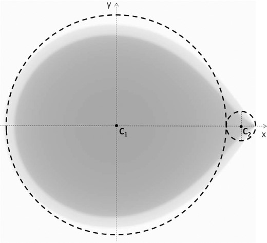
K-band mean intensity map given by the Roche lobe-filling model. The dashed large and small circles show the primary and the secondary components used by the spidast code for the binary model.
The calculated values for CSP are reported in Table 4. For a secondary-component temperature of 3200 K, the closest binary CSP values to the tidally deformed star simulation values are obtained with ϕ2 = 2.98 mas, and ε2 = 12.90 mas. With these parameter values, the displacement of the photometric barycenter produced by the binary model is identical to that produced by the Roche lobe-filling model.
K band CSP values (in degree) obtained for the Roche lobe-filling model and the binary model (T2 = 3200 K) with the linear (A0-D0-H0) and the triangular (A0-D2-H0) configurations.
| Model | A0–D0–H0 | A0–D2–H0 | |
|---|---|---|---|
| Roche lobe-filling model | 39.5 | 41.0 | |
| Binary model with | |||
| ε2 (mas) | ϕ2 (mas) | ||
| 11.5 | 3.00 | 3.0 | 43.3 |
| 12.0 | 3.00 | 18.0 | 40.6 |
| 12.5 | 3.00 | 33.1 | 40.7 |
| 12.9 | 3.00 | 39.9 | 41.3 |
| 12.9 | 2.99 | 39.7 | 41.2 |
| 12.9 | 2.98 | 39.6 | 41.1 |
Let us notice that we succeeded in matching the CSP values given by the complex model with the linear and the triangular configurations, by varying the values of the two parameters ϕ2 and ε2 of the binary model, while the three other parameters ϕ1, T2, and θ2 are kept fixed (the temperature of the primary being fixed by the selected atmospheric model). Choosing other values for the three fixed parameters leads to other values for the two free parameters, matching the input CSP values as well. Hence, the uniqueness of the values of the parameter set matching the CSP values is not guaranteed. This is illustrated in Fig. 4, where different parameter sets can produce the same CSP value. What is more, we claim that models producing the same displacement of the photometric centre produce the same CSP values.
When faced with a source with no a priori guess about its geometry, we anticipate that it might be difficult to find toy-models matching the observed CSP values. We stress that neither CSP nor GCP can discriminate between the model kind (i.e. binary or one-spot); however, they give an idea about the magnitude of the displacement of the photocentric barycentre with respect to the geometric one, which is nevertheless a valuable piece of information.
7 COMPARING THE ONE-SPOT MODEL TO STELLAR CONVECTION MODELS
Three-dimensional radiative-hydrodynamical (RHD) simulations carried out with the co5bold code (Freytag et al. 2012) show that evolved massive RSGs are characterized by large convective cells producing photospheric patterns (more noticeable in the infrared than in the visible) with a typical size comparable to the stellar radius, and evolving on a time-scale of tens of years (Chiavassa et al. 2009, 2010a,b, 2011b). On top of these cells, small convective structures (most conspicuous in the visible), with a size of about 5 to 20 per cent of the stellar radius, evolve on time-scales of weeks to months. The latter features result from the opacity variation and the gas dynamics at optical depths smaller than unity, i.e., farther up in the atmosphere with respect to the continuum-forming region (Chiavassa et al. 2011a).
The predicted granulation pattern causes SBAs, shown in Fig. 6, that are responsible for deviations from centrosymmetry (already measured in detail with closure phases and visibilities in the works by Chiavassa et al.). These departures can be mimicked by a simple geometrical model (one-spot) yielding (nearly) the same CSP value. The search for such a geometrical model is done in the following way.
We compute intensity maps at each wavelength of the AMBER MR–K band from the RHD simulation (denoted st35gm03n07), using the appropriate radiative transfer code optim3d (Chiavassa et al. 2009). The stellar parameters selected for the RHD simulation are: Teff = 3487 K, log g = −0.335, R = 830 R⊙, and M = 12 M⊙ (Chiavassa et al. 2011b). For each wavelength, we fit the actual instrumental resolution (|${\scr {R}=1500}$|) by using the appropriate top-hat filter on the set of wavelengths given by the RHD simulation. The simulation is scaled to an apparent angular diameter of 10 mas and the intensity maps are rotated by an angle of 71°, so that the direction of the shift of the large spot is aligned on the direction of the linear configuration.
We compute the 2D Fourier Transform of each monochromatic intensity distribution, as well as the triple product and the final CSP value as defined in equation (5). The calculations are made using the method explained in Chiavassa et al. (2009) and for the two configurations A0–D0–H0 (linear) and A0–D2–H0 (triangular).
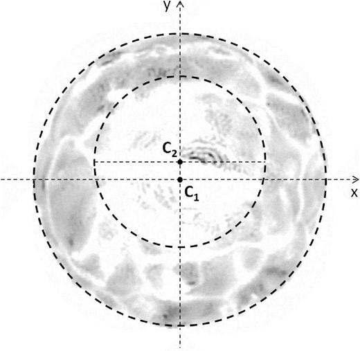
Infrared intensity map given by the hydrodynamic model, after removing the spatial frequencies lower than the first lobe of the visibility function (figure taken from Chiavassa et al. 2010b, see there for details). The dashed outer and inner circles show the approximate limits of the star and of the central convective cell, respectively.
In order to compare the values given by the spidast code using a one-spot model and the ones given by the RHD simulation, we perform the following steps.
We use a central marcs limb-darkened stellar disc of diameter ϕ1 = 10 mas with atmospheric parameters (extracted from a grid of models) as close as possible to the parameters used for the RHD simulation. The values we adopt are: T1 = 3490 K, log g = −0.6, M = 12 M⊙, [Fe/H] = 0.0, [α/Fe] = 0.0, and ξturb = 2 km s−1 (microturbulence velocity).
We add a blackbody spot with parameters: T2 = T1 = 3490 K,2 ϕ2 = 6 mas, ε2 = 0.6 mas, and θ2 = 71°. These values come from the intensity map of Fig. 6, where we point out the presence of a large central convective cell with a diameter of about 60 per cent the stellar diameter, slightly shifted upwards of about 6 per cent with respect to the stellar centre.
For various spot temperatures T2 in the range ±200 K around the disc temperature T1, we slightly vary the size ϕ2, the position ε2, in order to match the CSP values given by the RHD simulation with the same interferometric configurations A0–D0–H0 and A0–D2–H0.
The resulting values for the comparison are reported in Table 5. Since the initial parameters of the one-spot model have been chosen so as to reproduce the intensity map of the RHD simulation, the initial CSP values given by the one-spot model (40° with A0–D0–H0 and 16° with A0–D2–H0) are close to the CSP values given by the RHD simulation (43| $_{.}^{\circ}$|6 and 21| $_{.}^{\circ}$|8 , respectively). Note that the asymmetry in the one-spot model is the result of both the different fluxes for the blackbody and marcs models (due to line-blanketing, and despite the identical spot and disc temperatures) and the limb darkening whose point-symmetry has been broken by the presence of the non-centred spot.
K-band CSP values (in degree) obtained for the hydrodynamic model and the one-spot model with the linear (A0-D0-H0) and the triangular (A0-D2-H0) configurations.
| Model | A0–D0–H0 | A0–D2–H0 | ||
|---|---|---|---|---|
| 3D hydrodynamic model | 43.6 | 21.8 | ||
| one-spot model with | ||||
| T2 (K) | ε2 (mas) | ϕ2 (mas) | ||
| 3490 | 0.60 | 6.00 | 40.0 | 16.0 |
| 3490 | 0.72 | 5.88 | 43.6 | 21.6 |
| 3590 | 0.72 | 5.89 | 43.5 | 21.8 |
| 3690 | 0.72 | 5.90 | 43.7 | 21.6 |
| 3390 | 0.73 | 5.86 | 44.0 | 21.9 |
| 3290 | 0.73 | 5.84 | 43.8 | 21.9 |
Thus, the exact match of the 2 CSP values given by the RHD simulation can be easily achieved, thanks to the variation of the two parameters ϕ2 and ε2 of the one-spot model. Whatever the spot temperature, the closest one-spot CSP values to the RHD-simulation values are obtained with ϕ2 = 5.88 mas, and ε2 = 0.72 mas. Here again, we notice the small variation of the CSP values with respect to the spot temperature (see Section 4.2 for explanation).
Let us also note that, if we start with a different PA θ2 of the spot, we do not converge to a pair of (ϕ2,ε2) values matching the CSP values given by the RHD simulation. For instance, for θ2 = 0° (instead of 71°), the one-spot model with ϕ2 = 6.0 mas and ε2 = 0.6 mas gives CSP = 13| $_{.}^{\circ}$|2 with A0–D0–H0, and 39| $_{.}^{\circ}$|2 with A0–D2–H0, too far from the RHD-simulation CSP values of 43| $_{.}^{\circ}$|6 and 21| $_{.}^{\circ}$|8 , respectively.
In this section, we have shown that we can recover the CSP value given by the 3D hydrodynamic model by using the one-spot model. This, unsurprisingly, enhances the remark given in the previous section that models with similar geometries produce similar CSP values, although the opposite is not true.
We must emphasize that the one-spot model is a very crude way to represent the complex photospheric structures. More than one spot should be taken into account as well as proper intensity contrast and shape variations. However, as shown in (e.g.) Chiavassa et al. (2010b), fine surface inhomogeneities are associated with high spatial frequencies, appearing farther than the second visibility lobe, and they escape our capabilities in spatial resolution, since we only have information in the first and second lobes of the visibility curves. Thus, in the case of targets with small enough apparent diameter (i.e. where the details of the photospheres are not resolved), the one-spot model can be used to approach the stellar aspect given by the RHD simulation.
Let us note that with an actual (observed) source, we are not totally unaware of what is its physiognomy, and, for example with red giants and supergiants, a brightness distribution comprising one or several spots is rather commonplace. Besides, simple geometrical toy-models involve only few parameters. Thus, a fitting process, based on trials, is not totally blind at start, and the space of parameters to explore is rather limited, so that finding a satisfactory adjustment is not as hopeless as can be thought at first. Indeed, as already mentioned, observations from several configurations yield constraints which help to limit the range of variation for the geometrical parameters of the toy-model and the search for the best adjustment. Besides, a grid of ‘images’ computed from RHD simulations with various physical parameters, is available. Then, as soon as, for example, a one-spot toy-model is found relevant (agreement between observed and modelled CSP) the closest ‘image’ is selected as a first-level hypothetic representation of the observed source. The associated physical parameters can be considered as first estimates for iterative fine tuning of the RDH simulation leading to the final physical source parameters.
8 CONCLUSION
We have described the CSP, an indicator of deviation from centrosymmetry, for the study of source brightness asymmetries. To study its relevance, we have conducted several tests in parallel to the usual indicator called GPC (global phase closure). CSP takes advantage of the spectral information available over the whole set of individual channels in the spectral range given by a photometric filter.
To test the efficiency of CSP to measure the degree of asymmetry, we used models of brightness distribution which present known asymmetries, from which both GCP and CSP were calculated. The models are simple geometrical toy-models (binary model and the so-called one-spot model). This analysis showed that CSP is fully relevant for the detection of asymmetries and moreover that CSP is able to detect asymmetries that are not detected by GCP. Besides, CSP is more stable than GCP.
The second part of our study involved less simple models (physical Roche lobe model and hydrodynamical model) for which CSP was calculated. We showed that the simple toy-models can be a crude approximation of the brightness distributions provided by the physical models. In this attempt, CSP (associated with the simple models) works as a likeness tracer, and modifying the parameters of the simple models allows us to approach the target CSP value. Here must be recalled that, with an unknown brightness distribution, neither CSP nor GCP are able to infer a definite description and their role is at first limited to detection.
Fitting a simple model on an observed brightness distribution could bring some indications on the physiognomy of the source, but it can be thought hopeless to find applicable parameters. However, adjusting simple models on a real distribution involves only a few parameters, and moreover, if we combine observations with various interferometric configurations, additional constraints apply in the adjustment procedure. Therefore, there is some hope that suitable parameters of the simple model can be found.
In summary, we have shown that CSP is an efficient indicator for source brightness asymmetries, and yields a measure of the degree of asymmetry. It is complementing the use of GCP by additional capabilities. Moreover, it seems possible to use it as a help to build simple geometrical models, which could fit (at least roughly) to brightness distributions of observed sources via an iterative process involving physical and more complex models.
DEDICATION
This work is dedicated to the memory of our colleague and friend Olivier Chesneau, who prematurely deceased on 2014 May 17, at the age of 42. We miss his competence and enthusiasm.
We are grateful to the reviewer, Dr. S. Ragland, and to the Scientific and Assistant Editors for their constructive comments. PC thanks Emeritus Professor F. Rouviere from Nice University for helpful clarifications on partial differentiation of definite integrals with unconstant limits. CP is a PostDoc fellow supported by the Belgian Federal Science Policy Office via the PRODEX Programme of ESA. CS and GS thank Belspo and ESA Prodex for the financial support.
Deceased 2014 May 17.
acronym of SPectro-Interferometric Data Analysis Software Tool
Despite identical temperatures, the blackbody and marcs-model fluxes differ by about 20 per cent due to line-blanketing.
REFERENCES
APPENDIX A: ANGULAR AND RADIAL BOUNDARIES OF THE ELLIPSE
We describe hereafter the steps leading to the expressions of the boundaries in the standard case of an elliptic spot not truncated by the stellar limb
We start with θ2 equal to zero. We keep the same notations for the boundaries (r± and θ±), but we momentarily introduce 2A for the major axis (thus parallel to the y-direction, A = ϕ2/2) and 2B for the minor axis (B = μϕ2/2).
We determine the Cartesian coordinates of the points Q− and Q+, as well as the ones of the contact points of the tangent (setting the angular boundaries θ− and θ+).
We transform the Cartesian coordinates into polar coordinates.
Then, we consider the case θ2 ≠ 0, and the effect of changing this orientation will be done by a shift applied to the angular coordinates.
