Probing different regimes of strong field light–matter interaction with semiconductor quantum dots and few cavity photons

At its most essential level, light–matter interaction is based on the exchange of single energy quanta between a quantum oscillator and a photonic mode. For many applications in the field of quantum information processing an efficient coupling of flying (photons) and stationary (atoms) qubits is of fundamental importance. Semiconductor quantum dots (QDs) serve as ideal, artificially grown atomic qubits as they intrinsically provide a strong nonlinearity on the single-photon level enabling the generation of single-photon Fock states [1], indistinguishable photons [2] and entangled photon pairs [3]. Their integration into semiconductor microcavities enables high outcoupling efficiencies, reduction of the radiative lifetime due to Purcell enhancement, and coherent energy exchange between light and matter states in the strong coupling regime [4–11]. Regarding the interaction of flying and stationary qubits, cavities possess tremendous potential due to the enhanced light–matter coupling, low cavity losses and the high coupling efficiency to optical modes. Thus, all-optical switching with low-photon numbers [12], optical nonlinearities for few-photon pulses [13], single-photon filters [14], photon-sorters [15], and coherent manipulation of QDs with few photons [16] have been achieved.

The interaction between a strong oscillating electric field and a two-level system (TLS) strongly relies on the energy detuning between the two systems. In the resonant case the system can be described in the dressed states picture [17], where strong light–matter interaction leads to the formation of new, hybridized eigenstates. Using QDs as artificial atoms, these dressed states have been experimentally demonstrated either by the formation of the well-known Mollow triplet in photoluminescence (PL) spectroscopy [18–21] or by exploring the Autler–Townes splitting [22–25]. In the asymptotic limit of large detunings, the energy shift of the TLS can be described as a residual effect of the dressed states—known as the AC Stark shift [17, 26–28].

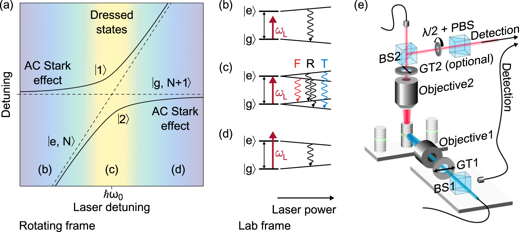
In this work, we enable strong light–matter interaction via the electric field enhancement of only few photons inside the cavity. Usually such strong interaction is only achievable by using strong laser fields and thousands of photons [10, 29, 30]. We systematically investigate the transition from the resonant Mollow triplet regime to the linear AC Stark effect for a large number of cavity-driven semiconductor QD-micropillar systems (figures 1(a)–(d)). Due to the self-assembled growth, the QD energy levels are randomly distributed, enabling a detailed study of the light–matter interaction over a wide range of QD-cavity detunings and coupling strengths. In addition, we observe a rich spectrum of behaviors depending on the QD-cavity coupling strength and orientation of the QD axis relative to the linearly polarized cavity mode. In particular in the resonant, case a single cavity photon mediates strong light–matter interactions resulting in a Mollow triplet with a sideband splitting of up to 45 μeV. Additionally, the appearance of an unexpected anomalous shift, i.e., towards the laser energy, is intuitively and qualitatively explained by a dressed 4-level model, which also includes the biexciton state. All experimental findings are well reproduced by a rigorous polaron master equation approach including QD-cavity coupling, electron–photon and electron–phonon scattering.

Zoom In Zoom Out Reset image size

The sample under investigation is grown by molecular beam epitaxy, and the self-assembled In${}_{0.45}$Ga${}_{0.55}$As QDs are embedded in a high-Q micropillar resonator, which consists of a GaAs λ-cavity confined by 26 and 30 pairs of distributed Bragg reflectors (DBRs) on the top and the bottom, respectively. These DBRs are composed of alternating $\lambda /4$ thick layers of GaAs and AlAs. The QD density of roughly ${10}^{10}\,{{\rm{cm}}}^{-2}$ and the wide spectral distribution due to the self-assembled growth enable the simultaneous investigation of several dots with various QD-cavity detuning and coupling strengths within one single micropillar. An aluminum mask on top of the micropillars reduces the scattered laser light in the case of resonant cavity pumping. We mount the sample inside a helium flow cryostat to perform micro-PL measurements at 7 K. Two microscope objectives (${\rm{NA}}=0.45$) in orthogonal configuration allow for excitation and detection from both the top and the side of the micropillar (figure 1(e)). The stray-light suppression is further improved by a pair of crossed polarizers in front of the objectives with a nominal suppression of 10⁵. We analyze the emission properties using a spectrometer with a 1800 l mm^–1 grating and a spectral resolution of 24 μeV. Using a $\lambda /2$-waveplate and a polarizing beamsplitter in front of the spectrometer we can perform polarization resolved micro-PL using the top detection path. For this purpose, we replace the polarizer for laser suppression with a longpass filter to clean up the resonant scattered laser light. By rotating the $\lambda /2$-waveplate we can then distinguish between the two linear polarized exciton states $| X\rangle$ and $| Y\rangle$ due to their perpendicular polarized light emission.

In order to gain detailed insight into the light–matter interaction we investigate more than 400 QDs in about 15 micropillars with a diameter of 1.5 μm. Almost all cavities exhibit two non-degenerated, orthogonally polarized fundamental modes (FMs) due to the elliptical shape of the micropillar [31]. The quality factors are between 14 000 and 19 000 estimated by the measured cavity linewidths. Intuitively, one can interpret the quality factor Q as the average number of roundtrips a photon makes before leaving the cavity. The use of a cavity strongly enhances the electrical field for each photon and thus reduces the total number of photons needed compared to free-space experiments. In the following experiments, we couple a resonant, linearly polarized continuous wave (CW) laser with a linewidth smaller than 2 MHz into one of the polarized FMs, i.e., from the top of the pillar. The QD emission is then collected from the side of the micropillar.

We investigate the influence of the cavity-enhanced light field on the QD states by micro-PL measurements as a function of the incident laser power. A color-scale map of the PL intensity in dependence of the emission energy ${\hslash }\omega$ with respect to the cavity mode ${\hslash }{\omega }_{c}$, and the laser power is plotted for two different, representative QD-micropillar systems in figure 2 to demonstrate various light–matter interaction effects. Firstly, the QD emission is distributed over a large spectral range, thus enabling an extensive study. Secondly, for mostly all resonantly driven cavities the emission at lower energy side of the cavity is more pronounced due to a more probable phonon excitation than absorption at low temperatures (see Micropillar 1 in figure 2). Thirdly, we observe a clear tendency of almost all emission lines shifting away from the cavity with increasing pump power—most lines shift linearly, but some lines also exhibit a nonlinear shift with increasing pump fields.

Zoom In Zoom Out Reset image size

The red boxes in figure 2 highlight some exemplary line shifts depending on the detuning and the QD orientation with respect to the cavity axes. In the next sections we further analyze these highlighted lines amongst others, which are not displayed in figure 2.

3.1. Small detuning: dressed-states regime

When the QD exciton-to-ground state transition nears resonance with the cavity mode and the driving laser, the occurrence of dressed states—essentially observable through the Mollow triplet sidebands in PL spectroscopy—is a signature of strong coupling of light and matter states (see figures 1(a) and (c)). The normalized color-scale plot in figure 3(a) displays power dependent PL measurements and visualizes clearly the appearance of two sidebands, i.e., the Fluorescence Line (F) and the Three Photon Line (T). The Rabi splitting ${{\rm{\Omega }}}_{x}$ is additionally plotted in figure 3(b) and grows linearly with the square root of the applied laser power, which is proportional to the Rabi frequency Ω_c driving the cavity mode. Here, we reach Rabi splittings of up to 295 μeV for an incident laser power of 5.62 μW ($\sqrt{P}=2.37\,\sqrt{\mu {\rm{W}}}$), not limited by any physical issue but due to spectral overlap with other QDs. In the limit of a strongly driven weakly coupled cavity we can adiabatically eliminate the cavity mode by a coherent state $\alpha =2{\eta }_{c}/\kappa$ [32, 33], with the cavity decay rate ${\hslash }\kappa$ = 74 μeV and the direct cavity drive ${\eta }_{c}$, which is twice the Rabi frequency ${{\rm{\Omega }}}_{c}$. We assume the cavity photon number to be very close to ${| \alpha | }^{2}={\left(\tfrac{2{\eta }_{c}}{\kappa }\right)}^{2}$ as the cavity is primarily driven by the laser with ${\eta }_{c}$. We can then estimate the mean cavity photon number as follows:

$$\begin{eqnarray}&&\langle {n}_{c}\rangle ={\left(\displaystyle \frac{2{\eta }_{c}}{\kappa }\right)}^{2}={\left(\displaystyle \frac{{\eta }_{x}}{\langle B\rangle g}\right)}^{2}={\left(\displaystyle \frac{{{\rm{\Omega }}}_{x}}{2\langle B\rangle g}\right)}^{2}.\end{eqnarray} \tag{ 1 }$$

The effect of the cavity on the QD can be represented as an off-resonant exciton drive ${\eta }_{x}=\langle B\rangle g\alpha$ [33], where $\langle B\rangle$ is the thermally averaged coherent phonon bath displacement operator [34–36]. For the given temperature of 21 K for this particular resonant measurement $\langle B\rangle =0.91$. The optimal QD-cavity coupling strength is given by ${\hslash }g={[({e}^{2}f)/(4{n}^{2}{\epsilon }_{0}{m}_{e}V)]}^{1/2}$ ≈ 35 μeV with an oscillator strength $f\approx 10$ for a typical lifetime of ${{T}}_{1}=1.2$ ns, an effective mode volume $V\approx 0.23\,\mu {{\rm{m}}}^{3}$ [4] and the refractive index n of the surrounding semiconductor material. However, for the calculations, we use an intermediate QD-cavity coupling strength of 25 μeV which reflects different polarization and spatial displacement of the QDs within the cavity (compare figure 4(d)). Thereby, we ensure to not underestimate the average cavity photon number $\langle {n}_{c}\rangle$. It is displayed in figure 3(b): only a few cavity photons are necessary for substantial Rabi splittings ${{\rm{\Omega }}}_{x}$ of the exciton transition. More important is the measured Rabi splitting of 45 μeV for a single cavity photon, which is several times larger than the natural linewidth of a typical InAs QD. Thus, the QD exciton state can be used to probe genuine quantum fields at the few photon limits.

Zoom In Zoom Out Reset image size

Zoom In Zoom Out Reset image size

Note: the sideband's linewidth exhibits an almost linear increase with excitation power due to an increased carrier-phonon coupling, which causes excitation-induced dephasing (EID). This has been reported for different not cavity-driven systems and is thus not subject of our investigation [37–39].

If the driving laser is off resonance with the TLS, the frequencies of the three Mollow triplet emission lines, in the strong field limit, are given by [20, 40, 41]

$$\begin{eqnarray}{\omega }_{\mathrm{central}} & = & {\omega }_{0}-{\rm{\Delta }},\\ {\omega }_{\mathrm{side}} & = & {\omega }_{0}-{\rm{\Delta }}\pm {\rm{\Omega }}.\end{eqnarray} \tag{ 2 }$$

Here, ${\omega }_{0}$ is the bare two-level transition frequency, ${\rm{\Delta }}={\omega }_{0}-{\omega }_{L}$ is the laser frequency detuning, and ${\rm{\Omega }}=\sqrt{{{\rm{\Delta }}}^{2}+{{\rm{\Omega }}}_{x}^{2}}$ is the effective Rabi frequency. It is worth mentioning that the detuning Δ is defined as the QD emission frequency with respect to the fixed laser frequency. In the literature, this detuning is normally defined as the opposite value, because the laser frequency is tuned with respect to a single TLS frequency. In most of the following experiments the laser frequency will be fixed at the cavity frequency and QDs with different QD-cavity detuning will be investigated. In the case of a strictly resonant interaction the sidebands shift linearly with the bare Rabi frequency ${{\rm{\Omega }}}_{x}$, as presented before.

First we tune the laser ($\sqrt{P}=0.84\,\mu {{\rm{W}}}^{1/2}$) with respect to the cavity mode and plot the normalized PL intensity of the Mollow triplet in figure 3(c). The three emission lines exhibit a distinct anticrossing, which differs in shape from the anticrossing of coherently driven non-cavity systems (given by the dashed lines in figure 3(c)). This is due to the spectral filtering of the cavity mode itself, i.e., the number of photons entering the cavity strongly depends on the detuning between laser and cavity. Thus, a detuned laser results in a reduced bare Rabi frequency driving the cavity. The line shift and also the anticrossing is then superimposed with an effective Rabi field from the cavity mode:

$$\begin{eqnarray}&&{\rm{\Omega }}=\sqrt{{{\rm{\Delta }}}^{2}+{(F({\rm{\Delta }})\cdot {{\rm{\Omega }}}_{x})}^{2}},\end{eqnarray} \tag{ 3 }$$

where the factor $F({\rm{\Delta }})=\tfrac{1}{1+{\left(\tfrac{{\rm{\Delta }}}{\kappa /2}\right)}^{2}}$ accounts for the spectral filtering from the cavity mode. In figure 3(c) we used this equation to fit the detuning dependence of the Mollow triplet sidebands (solid lines). The dashed lines represent the lines detuning dependence for the same Rabi frequency but without cavity filtering. For a more convenient study, we extract the total splitting between the two sidebands and plot the results in figure 3(d). From a least-squares fit $\propto 2\sqrt{{{\rm{\Delta }}}^{2}+{(F({\rm{\Delta }})\cdot {{\rm{\Omega }}}_{x})}^{2}}$ to the data, we derive a bare Rabi frequency of ${\hslash }{{\rm{\Omega }}}_{x}=117\,\mu$ eV (${{\rm{\Omega }}}_{x}/(2\pi )=28.2\,$ GHz) for zero detuning. This driving field is generated by only a mean cavity photon number of 6.6.

We now investigate the power dependence of the line shift for larger QD-cavity detunings (the laser is again resonant to the cavity mode). The relative line shift for several QDs with different positive and negative detuning with respect to the cavity mode as a function of the applied laser power is displayed in figure 3(e). Besides the large differences in strength, which strongly depends on the detuning, the line shifts also differ in the form of their power dependence. We use equation (2) to fit the energy detuning, represented by the solid lines. The transition from strongly dressed states (0 meV detuning, already discussed in detail in figures 3(a) and (b)) with an energy shift proportional to the square root of the applied power to the linear AC Stark effect (3.8 meV and −2.7 meV) with an energy shift proportional to the applied power is clearly observable.

In the following section, we will further investigate the AC Stark effect and its detuning dependence in detail.

3.2. Asymptotic limit for large QD-laser detuning: AC Stark effect

For large QD-laser detuning, only the emission line close to ${\omega }_{0}$ of the Mollow triplet is still observable, as the admixture of light and matter states is strongly reduced [17]. We can then use a Taylor expansion of equation (2) to obtain a simple form for the expected AC Stark shift,

$$\begin{eqnarray}&&{\omega }_{{\rm{AC}}}\approx {\omega }_{0}+\displaystyle \frac{1}{2}\,\displaystyle \frac{{{\rm{\Omega }}}_{x}^{2}}{{\rm{\Delta }}},\end{eqnarray} \tag{ 4 }$$

which predicts the spectral line shift of the original TLS transition with frequency ${\omega }_{0}$. This AC Stark shift depends linearly on the applied laser power $P\propto {{\rm{\Omega }}}_{x}^{2}$, and is inversely proportional to the QD-laser detuning Δ. The sign of the detuning determines the direction of the energy level shift.

Typical linear line shifts for two QDs are plotted in figure 4(a) (box 1 in figure 2). Both emission lines are shifted negatively by roughly 150 μeV due to the AC Stark effect. At the same time the lines are broadened from 30 to 110 μeV due to EID (not shown here).

Some lines exhibit a splitting with increasing excitation power as shown for two QDs in figure 4(b) (box 2). The polarization resolved PL spectroscopy in figure 4(c) identifies two mainly linearly and perpendicularly polarized components for each emission line. Thus, we relate the splitting to the two exciton eigenstates $| X\rangle$ and $| Y\rangle$ from the same QD with orientation not parallel to the cavity axes. The corresponding QD transitions are now exposed to different Rabi oscillations, expressed by different cavity coupling strengths g_X and g_Y. The increase of the fine structure splitting from few μeV to more than 120 μeV reveals a considerably larger tuning range compared to non-cavity-driven semiconductor QD systems [24, 28].

With increasing laser power most emission lines exhibit the expected shift predominantly away from the cavity, i.e., negative for negatively detuned emission lines and positive for positively detuned emission lines. We fitted the energy shift for more than 400 QDs in 15 different cavities as a function of the applied laser power with the linear relation ${\rm{\Delta }}E=m\,P$. The slope $m\,(\mu \mathrm{eV}/\mu {\rm{W}})$ is then plotted in figure 4(d) as a function of the QD-cavity detuning. First of all, we clearly observe an inversely proportional dependence on the detuning, as expected from equation (4). The large variation in the strengths of the Stark shift for same detuning results from different QD-cavity couplings strengths, due to the QD oscillator strength, and the QD orientation and displacement inside the micropillar. However, it appears that a maximum coupling strength causes a sharp upper limit of the observable Stark shift. To calculate the Stark shift we insert equation (1) into equation (4) and exploit the relation of incident laser power and cavity photons in the steady state $\langle {n}_{c}\rangle ={\eta }_{{\rm{in}}}{P}_{{\rm{inc}}}/(\kappa \cdot {\hslash }\omega )$. ${\eta }_{{\rm{in}}}\approx 0.2$ is the coupling efficiency into the FM and can be obtained experimentally (figure 3(b)). The solid lines in figure 4(d) display the calculated Stark shift as a function of the detuning for different QD-cavity coupling strength (10 μeV–35 μeV). The optimal coupling strength of 35 μeV serves as upper limit of the measured values. Because of aforementioned reasons, most QDs exhibit a weaker Stark shift. The AC Stark shift per cavity photon number is explicitly given in figure 4(d), right y-scale. Apparently, a large number of cavity photons is necessary for the observed shifts of up to 150 μeV, because of the extraordinary large QD-cavity detuning.

For small detunings the AC Stark shift approximation (equation (4)) deviates from the analytic equation (2). The grey area in figure 4(d) indicates the detuning range with a deviation of more than 10% for a maximum bare Rabi frequency of 1.0 meV. For detunings smaller than 1.5 meV both the calculated and the experimentally collected slopes must be treated with caution, especially for large QD-cavity coupling strengths. For small detuning the number of investigated QDs decreases as the linear AC Stark effect is not valid any more, and most QDs show a nonlinear power dependence (see figures 3(e), (f)).

Most shifts in figure 4(d) reflect the expected AC Stark shift relation in equation (4), but some lines reveal an unexpected opposite Stark shift, i.e., they shift to higher energies although the QD-cavity detuning is negative, and vice versa. The related slopes are then located in the upper left and lower right quadrant of the graph (figure 4(d)). One example is highlighted within box 3 in figure 2, and a close-up view is given in figure 5(b). Although this particular emission line is positively detuned with respect to the cavity mode and the driving laser energy, one of the emerging lines exhibit a negative shift with increasing power. This anomalous shift can be explained by a detuned 4-level system, including the biexciton state $| {XX}\rangle$, the two exciton states $| {X}\rangle$, $| {Y}\rangle$, and the ground state $| {G}\rangle$. The level energy diagram is illustrated in figure 5(a, left). Here, the driving laser frequency is red detuned, i.e., the laser energy is smaller than all involved transitions. Due to the biexciton binding energy E_B the laser is spectrally closer to the biexciton emission energy ${\hslash }{\omega }_{{XX},X/Y}$ than to the exciton emission energy ${\hslash }{\omega }_{X/Y,G}$. Therefore, the former transition is initially shifted stronger by the light field as we have seen in figure 4(d). By calculating the new eigenstates ($| 1\rangle$–$| 4\rangle$) of the dressed 4-level atom [33], we can easily simulate their power dependence as depicted in figure 5(a, right) in the frame of the rotating laser. Note that the polarization of the laser also imposes its polarization on the mixed states, thus leading to the same eigenstates under strong drive and for a small fine structure splitting of the exciton levels. For convenience, we assume a linear polarized laser in x-direction, i.e., the effective drive of the y-polarized transitions is zero (${\eta }_{Y}={\eta }_{{YY}}=0$). The transition between $| 2\rangle$ (former state $| {X}\rangle$) and $| 1\rangle$ ($| {G}\rangle$) apparently exhibits a negative shift for small pump power. In other words: the strong dressing of the biexciton transition induces a negative shift of the more detuned exciton transition.

Zoom In Zoom Out Reset image size

The appearance of the anomalous shift and its strength strongly relies on the QD energy levels and their detuning with respect to the driving laser. The absolute value of this shift ${{\rm{\Delta }}}_{\mathrm{anom}}$ is plotted in figure 5(c) as a function of the exciton detuning ${{\rm{\Delta }}}_{{xL}}={\hslash }({\omega }_{x}-{\omega }_{L})$ and the biexciton binding energy E_B. It occurs within two separated regions of the parameter space where one is located around the biexciton resonance condition (${{\rm{\Delta }}}_{{xL}}={E}_{B}$). It covers all cases that exhibit a negative shift of one exciton emission line including the presented experimental case for an exciton detuning of 6.7 meV (figure 5(b)). The appropriate biexciton binding energy is roughly 4 meV for this special detuning and the measured negative shift, a reasonable value for InAs QDs. We actually find a weak emission line with the correct detuning in figure 2, but cannot definitely assign it to the biexciton transition due to strong spectral overlap with other emission lines. The anomalous shift of the exciton transition reaches its maximum for resonant biexciton drive. The second region is located around the exciton resonance (${{\rm{\Delta }}}_{{xL}}=0$). Here, one of the biexciton-to-exciton transitions is shifted to higher energy, although the laser is located at higher energy. This anomalous shift is the direct counterpart of the presented data. The two regions are symmetric to the two-photon resonance condition (${{\rm{\Delta }}}_{{xL}}={E}_{B}/2$) highlighted with the yellow dashed line in figure 5(c).

The required pump power (${{\eta }_{x}}^{2}$) to reach the maximum anomalous line shift is plotted in figure 5(d) for the same parameter space.

4.1. Theoretical description and numerical simulations

We next discuss our theoretical model using a polaron master equation approach to calculate the anomalous Stark shift for this cavity-driven QD system, closely following the works of [32, 33, 36].

The biexciton-exciton system consists of four states, including the biexciton state $| {XX}\rangle$, $| X\rangle$ and $| Y\rangle$ polarized exciton states and the ground state $| G\rangle$. In contrast to [33] we assume that the polarization of the orthogonal QD transitions ($x^{\prime}$ and $y^{\prime}$) are not aligned with the orthogonal cavity modes (x and y) and rotated by an angle θ to better match the experimental measurements. The orthogonal $x^{\prime}$-polarized and $y^{\prime}$-polarized transitions of the QD namely $| {XX}\rangle$-$| X\rangle$, $| X\rangle$-$| G\rangle$ and $| {XX}\rangle$-$| Y\rangle$, $| Y\rangle$-$| G\rangle$ are coupled to both the orthogonal x- (y-) polarized cavities of the micropillar. The x-polarized cavity is driven by a coherent laser. The following Hamiltonian, written in the frame of the rotating laser, includes the four QD states, cavity driving, QD-cavity interactions, and electron–phonon interactions,

$$\begin{eqnarray}&&H={H}_{\mathrm{QD}}+{H}_{\mathrm{light}}+{H}_{\mathrm{int}}+{H}_{\mathrm{phonons}},\end{eqnarray} \tag{ 5 }$$

with

$$\begin{eqnarray*}{H}_{\mathrm{QD}} & = & {\hslash }{{\rm{\Delta }}}_{4}| {XX}\rangle \langle {XX}| +{\hslash }{{\rm{\Delta }}}_{3}| X\rangle \langle X| +{\hslash }{{\rm{\Delta }}}_{2}| Y\rangle \langle Y| ,\\ {H}_{\mathrm{light}} & = & \displaystyle \sum _{P=x,y}{\hslash }{{\rm{\Delta }}}_{{cL}}^{P}{a}_{P}^{\dagger }{a}_{P}+{\hslash }{\eta }_{c}({a}_{x}^{\dagger }+{a}_{x}),\\ {H}_{\mathrm{int}} & = & {\hslash }{g}_{2}^{x^{\prime} x}({\sigma }_{{XX}{\rm{-}}X}^{+}{a}_{x}+{a}_{x}^{\dagger }{\sigma }_{{XX}{\rm{-}}X}^{-})+{\hslash }{g}_{1}^{x^{\prime} x}({\sigma }_{X{\rm{-}}G}^{+}{a}_{x}+{a}_{x}^{\dagger }{\sigma }_{X{\rm{-}}G}^{-}),\\ & & +{\hslash }{g}_{2}^{x^{\prime} y}({\sigma }_{{XX}{\rm{-}}X}^{+}{a}_{y}+{a}_{y}^{\dagger }{\sigma }_{{XX}{\rm{-}}X}^{-})+{\hslash }{g}_{1}^{x^{\prime} y}({\sigma }_{X{\rm{-}}G}^{+}{a}_{y}+{a}_{y}^{\dagger }{\sigma }_{X{\rm{-}}G}^{-}),\\ & & +{\hslash }{g}_{2}^{y^{\prime} y}({\sigma }_{{XX}{\rm{-}}Y}^{+}{a}_{y}+{a}_{y}^{\dagger }{\sigma }_{{XX}{\rm{-}}Y}^{-})+{\hslash }{g}_{1}^{y^{\prime} y}({\sigma }_{Y{\rm{-}}G}^{+}{a}_{y}+{a}_{y}^{\dagger }{\sigma }_{Y{\rm{-}}G}^{-}),\\ & & +{\hslash }{g}_{2}^{y^{\prime} x}({\sigma }_{{XX}{\rm{-}}Y}^{+}{a}_{x}+{a}_{x}^{\dagger }{\sigma }_{{XX}{\rm{-}}Y}^{-})+{\hslash }{g}_{1}^{y^{\prime} x}({\sigma }_{Y{\rm{-}}G}^{+}{a}_{x}+{a}_{x}^{\dagger }{\sigma }_{Y{\rm{-}}G}^{-}),\\ {H}_{\mathrm{phonons}} & = & \displaystyle \sum _{q}{\hslash }{\omega }_{q}{b}_{q}^{\dagger }{b}_{q}+\displaystyle \sum _{S=X,Y,{XX}}| S\rangle \langle S| \displaystyle \sum _{q}{\hslash }{\lambda }_{q}^{S}({b}_{q}^{\dagger }+{b}_{q}).\end{eqnarray*}$$

The detunings Δ of the bare QD states and cavities are measured with respect to the driving laser frequency ${\omega }_{L}$. These detunings are labeled as ${{\rm{\Delta }}}_{4}={\omega }_{{XX}}-2{\omega }_{L}$ for the biexciton, ${{\rm{\Delta }}}_{3}={\omega }_{X}-{\omega }_{L}$ for the X exciton, ${{\rm{\Delta }}}_{2}={\omega }_{Y}-{\omega }_{L}$ for Y exciton, ${{\rm{\Delta }}}_{{cL}}^{x}={\omega }_{c}^{x}-{\omega }_{L}$ for the X-cavity and ${{\rm{\Delta }}}_{{cL}}^{y}={\omega }_{c}^{y}-{\omega }_{L}$ for the Y-cavity, where ${\omega }_{c}^{x,y}$ are the bare cavity frequencies. Here, the X and Y excitons are detuned by ${\delta }_{{XY}}$ due to a possible anisotropic exchange interaction. To be consistent with the experiments, the x-polarized cavity is driven by an x-polarized resonant laser with amplitude ${\eta }_{c}$ (two times the Rabi field) and frequency ${\omega }_{L}$. The operators ${a}_{x,y}$ describe lowering operators for x- and y-polarized cavities. The QD lowering operator ${\sigma }_{A{\rm{-}}B}^{-}$ denotes lowering from state $| A\rangle$ to $| B\rangle$. The four QD transitions are coupled to the two cavity modes with the coupling rates ${g}_{1,2}^{{ab}}$, where the superscript describes coupling between the a polarized QD transition with a b polarized cavity mode and the subscripts 2 and 1 denote biexciton-to-exciton and exciton-to-ground state transition, respectively. b_q (${b}_{q}^{\dagger }$) are the annihilation (creation) operators of the acoustic phonons and ${\lambda }_{q}$ is the exciton-phonon coupling strength.

Since we are in the weak-to-intermediate coupling limit, we can conveniently adiabatically eliminate the cavity and describe the state of the driven cavity as a coherent state, $\alpha =2{\eta }_{c}/\kappa$, with cavity decay rate κ [32, 33]. The effect of the cavity on the QD can be represented as an off-resonant exciton drive ${\eta }_{x}=\langle B\rangle g\alpha$ [33], where $\langle B\rangle$ is the thermally averaged coherent phonon bath displacement operator [34–36].

We subsequently derive an extended polaron master equation for the total biexciton-exciton system [33] which additionally contains extra spontaneous decay and dephasing rates for the various QD transitions as Lindblad terms, e.g., ${\gamma }_{{XX}{\rm{-}}X}$ is the radiative decay rate from the biexciton to the x-polarized exciton. The final master equation is used to calculate the y-polarized spectrum, measured in the experiment, which computed from [33]

$$\begin{eqnarray}&&{S}_{{y}}(\omega )=\sin (\theta ){S}_{{x}^{\prime} }+\cos (\theta ){S}_{{y}^{\prime} },\end{eqnarray} \tag{ 6 }$$

with ${S}_{{y}^{\prime} }(\omega )={\mathrm{lim}}_{t\to \infty }\mathrm{Re}[{\int }_{0}^{\infty }{\rm{d}}\tau (\langle {\sigma }_{Y}^{+}(t+\tau ){\sigma }_{Y}^{-}(t)\rangle -\langle {\sigma }_{Y}^{+}(t){\sigma }_{Y}^{-}(t)){{\rm{e}}}^{{\rm{i}}({\omega }_{L}-\omega )\tau }]$, ${S}_{{x}^{\prime} }(\omega )={\mathrm{lim}}_{t\to \infty }{\rm{Re}}[{\int }_{0}^{\infty }{\rm{d}}\tau (\langle {\sigma }_{X}^{+}(t+\tau ){\sigma }_{X}^{-}(t)\rangle -\langle {\sigma }_{X}^{+}(t){\sigma }_{X}^{-}(t)){{\rm{e}}}^{{\rm{i}}({\omega }_{L}-\omega )\tau }],$ where ${\sigma }_{X}^{-}={d}_{{XX}-X}{\sigma }_{{XX}-X}^{-}+{d}_{X-G}{\sigma }_{X-G}^{-}$, ${\sigma }_{Y}^{-}={d}_{{XX}-Y}{\sigma }_{{XX}-Y}^{-}+{d}_{Y-G}{\sigma }_{Y-G}^{-}$ and d_AB corresponds to the magnitude of the dipole moment connecting transition between states $| A\rangle$ to $| B\rangle$ and is determined from the bare spontaneous emission rate connecting these states, i.e., ${d}_{{AB}}\propto \sqrt{{\gamma }_{{AB}}}$.

For our calculations, we use a biexciton binding energy of 3 meV and the original single exciton-ground transition is located at 6 meV (=${\hslash }{{\rm{\Delta }}}_{{xc}}$) from the driven cavity, as in the measurement (see caption of figure 5 for detailed parameter description). Thus for low drives the exciton-to-ground and biexciton-to-exciton transitions are located at 6 and 3 meV, respectively (figure 5(e), red line). Strong dressing leads to 13 distinct lines in the total spectra which are symmetric to the laser frequency (figure 5(e), black line) [33]. The spectra are plotted in a log₁₀ scale for better visibility and two lines are still barely visible in the total spectra. Two lines apparently emerge from the exciton emission line at ${\rm{\Delta }}=6$ meV. In figure 5(f), we focus around the region of this exciton-to-ground state transition like in the experiment and connect with the observed experimental features (figure 5(b)). As it can be recognized, the experimentally observed line shifts are qualitatively reproduced. Especially the lower energy emission line's anomalous, negative shift is well-understood using our 4-level QD-cavity approach with a driving laser far detuned from the two-photon resonance condition of the biexciton state (compare for the results in [33]).

We have systematically investigated the transition from dressed states (Mollow triplet) to the AC Stark effect for a large number of cavity-driven semiconductor QD-micropillar systems. The self-assembled growth of the QDs allows for comprehensive study of the light–matter interaction over a wide range of QD-cavity detuning and coupling strengths. In the resonant case, we observe strong light–matter coupling on the single photon level. A Mollow triplet sideband splitting of up to 45 μeV is mediated by a mean cavity photon number of $\langle {n}_{c}\rangle =1$ due to the cavity-enhanced electric field. For a large detuning the QD energy shift shows linear dependence with applied laser power and an inversely proportional dependence with QD-cavity detuning, characterizing the linear optical Stark effect. Here, we investigated more than 400 QDs to account for statistical changes in the QD-cavity strengths due to the QD oscillator strength, and the QD orientation and displacement inside the micropillar. The appearance of an unexpected anomalous shift, i.e., towards the laser energy, is intuitively and qualitatively explained by a dressed 4-level system, which additionally includes the biexciton state. The experimental observation of this anomalous shift is successfully reproduced by an extended polaron master equation approach including QD-cavity coupling, electron–phonon and electron–photon scattering.

We thank M Emmerling for expert sample fabrication. We acknowledge financial support of the Deutsche Forschungsgemeinschaft (DFG) within the SFB/TRR21 and the projects MI500/23-1 and Ka2318/4-1,  the Natural Sciences and Engineering Research Council of Canada, and from the open access fund of the University of Stuttgart..

In this appendix, we discuss how the Stark shifts of the QDs are estimated, the validity of the adiabatic approximation for eliminating the cavity mode from the systems Hamiltonian, and the precise role played by phonons on the Stark shift.

The Stark shift of the QD due to the cavity pump ${\eta }_{c}$ is estimated from the shift of the zero phonon line of the QD as shown in figures 6(a), (b), where a 20 μeV Stark shift is applied on the QD (originally at 2.5 meV) for a negative (a) and positive (b) detuning ${{\rm{\Delta }}}_{{xc}}$. The dashed lines are exact simulations of the full polaron master equation approach introduced in [33] and explained for the 4-level model in the main text, while the solid lines show the spectra calculated using the adiabatic elimination [33] and they match the full numerical results (with no approximations) very closely. Thus, in the paper we have used this adiabatic approximation for all calculations shown. Specifically, we assume the cavity photon number to be very close to ${(2{\eta }_{c}/\kappa )}^{2}$ as the cavity photons are primarily driven by the direct drive ${\eta }_{c}$ and the drive required for implementing a Stark shift on an off-resonant QD is strong. This allows us to employ the adiabatic approximation on the cavity which substantially simplifies the numerical simulations. In the presence of a strong cavity drive ${\eta }_{c}$, a high photon number ($\gt 40$) is typically required for convergence, which makes the spectrum calculations numerically difficult. This can however be simplified in the following way: when a weak coupling condition between the QD and cavity is met and the cavity is driven strongly, the cavity can be adiabatically eliminated. In this limit, as stated in the main text, the state of the driven cavity can be described as a coherent state α and is given by $\alpha =2{\eta }_{c}/\kappa$ from the QD-cavity Bloch equations (in resonance case). The effect of the cavity on the QD can be represented as an off-resonant exciton drive ${\eta }_{x}=\langle B\rangle g\alpha$ [32, 33]. With the cavity adiabatically eliminated, the numerical simulations becomes significantly easier. In addition to a cavity-modified drive, the adiabatic elimination also introduces a cavity modified spontaneous emission enhancement through the Purcell effect. However, for the large detunings considered in this paper, the Purcell modification is negligible and thus not included.

Zoom In Zoom Out Reset image size

The spectrum for positive ${{\rm{\Delta }}}_{{xc}}$ normalizes both spectra in figures A1(a), (b), and the QD located to the left of the cavity reveals stronger excitation by the resonant cavity drive. This happens because phonon emission is stronger than absorption at low temperatures and a QD is coupled more strongly through phonon emission, when it has a lower energy than the cavity. Next, we study the influence of phonons on the spectral AC Stark shift.

The Stark-shift of the QD vs laser power (${\eta }_{c}^{2}$) is plotted in figure A1(c) using the adiabatic elimination, for a negative (black, solid) and positive (red, dashed) detuning ${{\rm{\Delta }}}_{{xc}}$, where $| {\hslash }{{\rm{\Delta }}}_{{xc}}|$ = 3.5 meV. Without phonon coupling, the drive amplitude ${\eta }_{c}(={{\rm{\Omega }}}_{c}/2)$ for a Stark shift ${{\rm{\Delta }}}_{S}$ is given by ${\eta }_{c}=\tfrac{\kappa }{g}\sqrt{\tfrac{| {{\rm{\Delta }}}_{S}{{\rm{\Delta }}}_{{xc}}| }{8}}$ and the slope $\left|\tfrac{{{\rm{\Delta }}}_{S}}{{\eta }_{c}^{2}}\right|=\tfrac{8{g}^{2}}{| {{\rm{\Delta }}}_{{xc}}| {\kappa }^{2}}$. The Stark shift without phonon contributions is also plotted in figure A1(c) (dotted, blue) and reveals almost no difference. The slope estimated from figure A1(c) is plotted for various detunings $| {{\rm{\Delta }}}_{{xc}}|$ in figure A1(d). Here the solid and dashed lines denote slopes for negative and positive ${{\rm{\Delta }}}_{{xc}}$ respectively and the Stark shifts and slopes are approximately the same. In addition, the calculations ignoring phonon effects are again in good agreement. For small detunings these simple calculations show a slight mismatch as the AC Stark effect approximation (equation (4)) deviates from the exact solution (equation (2)).

Finally, we assess the role of phonons at higher temperatures. Since at an elevated temperature of T $\approx$ 50 K, $\langle B\rangle$ (=0.71) is small ($\langle B\rangle$ = 0.96 at $T=4\,$ K) , the applied Stark shift due to effective drive ${\eta }_{x}=\langle B\rangle g\alpha$ is expected to be small through the coherent reduction of the drive. However a large phonon-mediated Lamb-shift at high T compensates for this effect and a large frequency shift is observed. This can be seen from figure A2, where the light solid line includes only the coherent contribution of phonons (${H}_{{S}}^{\prime }$) and ignores phonon induced fluctuations and the dark solid line shows full phonon calculations, where the phonon fluctuations gives rise to large Lamb shifts [36]. The dashed red line is calculations without phonon interactions.

Zoom In Zoom Out Reset image size