
ABSTRACT
For the very best and brightest asteroseismic solar-type targets observed by Kepler, the frequency precision is sufficient to determine the acoustic depths of the surface convective layer and the helium ionization zone. Such sharp features inside the acoustic cavity of the star, which we call acoustic glitches, create small oscillatory deviations from the uniform spacing of frequencies in a sequence of oscillation modes with the same spherical harmonic degree. We use these oscillatory signals to determine the acoustic locations of such features in 19 solar-type stars observed by the Kepler mission. Four independent groups of researchers utilized the oscillation frequencies themselves, the second differences of the frequencies and the ratio of the small and large separation to locate the base of the convection zone and the second helium ionization zone. Despite the significantly different methods of analysis, good agreement was found between the results of these four groups, barring a few cases. These results also agree reasonably well with the locations of these layers in representative models of the stars. These results firmly establish the presence of the oscillatory signals in the asteroseismic data and the viability of several techniques to determine the location of acoustic glitches inside stars.
Export citation and abstract BibTeX RIS
1. INTRODUCTION
Acoustic glitches in a star are the regions where the sound speed undergoes an abrupt variation due to a localized sharp change in the stratification. The major acoustic glitches are the boundaries between radiative and convective regions and the layers of ionization of elements, especially hydrogen and helium. Such a glitch introduces an oscillatory component, δν, in the eigenfrequencies of the star with respect to the frequencies themselves (Gough & Thompson 1988; Vorontsov 1988; Gough 1990), proportional to

where
is the acoustic depth of the glitch measured from the surface, c the adiabatic sound speed, rg is the radial distance of the glitch, Rs is the seismic radius of the star (see discussion below), νn, l is the frequency of a mode with radial order n and degree l, and ϕ is a phase factor. Each glitch will contribute to such a signal in the frequencies with a "periodicity" of twice the acoustic depth of the corresponding glitch.
This oscillatory signature has been extensively studied for the Sun in order to determine the extent of overshoot below the solar convection zone (Vorontsov 1988; Gough 1990; Gough & Sekii 1993; Monteiro et al. 1994; Basu et al. 1994; Roxburgh & Vorontsov 1994; Basu 1997; Christensen-Dalsgaard et al. 2011) and the seismic solar age (Houdek & Gough 2011).
It has been proposed earlier that this may also be used for distant stars to find the position of the base of the convective envelope or the second helium ionization zone (Monteiro et al. 2000; Mazumdar & Antia 2001; Gough 2002; Roxburgh & Vorontsov 2003; Ballot et al. 2004; Basu et al. 2004; Houdek 2004; Mazumdar 2005; Piau et al. 2005; Houdek & Gough 2006, 2007). Indeed, Miglio et al. (2010) used the modulation of the frequency separations to determine the location of the second helium ionization zone in the red giant star, HR7349, observed with the CoRoT satellite. Recently, Mazumdar et al. (2012) used the oscillatory signal in the second differences of the frequencies of the solar-type CoRoT target star, HD49933, to determine the acoustic depths of its second helium ionization zone and the base of the convective envelope (see also Mazumdar et al. 2011; Roxburgh 2011). Earlier, Bedding et al. (2010) reported detection of an acoustic glitch in Procyon, although no association to a specific layer was made.
The scientific interest in studying the acoustic glitches goes beyond the obvious goal of placing constraints on the positions of specific layers in the stellar interior. The accurate determination of the location and profile of the transition at the base of the convective envelope, for example, will help us refine our understanding of the stellar dynamo in cool stars. On the other hand, the amplitude of the oscillatory signal from the ionization zones is directly related to the abundance of the corresponding element in the star. For helium especially, an estimate of the helium abundance in an ensemble of stars of different masses and ages will lead us to a better understanding of the process of element enrichment in stars which can be extrapolated back to the primordial helium content of the universe, an important parameter in cosmology.
The acoustic glitches can be used to determine the acoustic depth of the surface convection zone in a star, which in turn can be used to constrain the stellar models. In particular, the position of the base of the convection zone is very sensitive to the opacity of stellar material, which depends on the heavy element abundances. It is well known that the recent determination of heavy element abundances (Asplund et al. 2009) using three-dimensional (3D) hydrodynamic atmospheric models for the Sun are not consistent with helioseismic data (Basu & Antia 2008; Gough 2013 and references therein). On the other hand, the older abundances of Grevesse & Sauval (1998) estimated using one-dimensional atmospheric models are consistent with helioseismic data. The cause of this discrepancy is not understood, and it would be interesting to test whether asteroseismic data are consistent with the revised abundances. In particular, the heavy element abundance, Z, for stars is estimated from the observed [Fe/H] ratio. Thus, the estimated value of Z depends on the heavy element mixture (ratio of Fe to H abundance) for the Sun. Recently, van Saders & Pinsonneault (2012), noting the dependence on Z of the acoustic depth of the convection zone, proposed that the measured acoustic depth can be used to constrain Z.
The effects of the acoustic glitches are subtle, and hence great care is required in ascertaining that the results of the analyses reflect the stellar properties at a significant level. Although analysis of artificial data (e.g., Basu et al. 2004; Mazumdar 2005; Monteiro & Thompson 2005; Houdek & Gough 2007) are useful in this regard, real data may well give rise to effects that are not contained in such simulations. Here, we test the reliability of the inferences by comparing the results of several independent fits to the glitch properties of the same frequency data, using rather different techniques. These all provide measures of the acoustic locations of the glitches which can be directly compared. Other properties of the fits, however, depend more sensitively on the techniques and hence can only properly be interpreted in the context of comparisons with model results. We return to this point in Section 6.
In the present analysis, we studied 19 stars continuously observed by the Kepler mission (Borucki et al. 2010; Koch et al. 2010) over nine months. Launched on 2009 March 7, Kepler is monitoring 150,000 stars in the constellations of Cygnus and Lyra every half an hour to look for Earth-like planets orbiting solar-like stars. Photometric time series of a subsample of 512 stars are studied at a shorter cadence of 58.8 s (Gilliland et al. 2010). Every three months, the spacecraft rolls by 90° to maintain the solar panels directed toward the Sun. Therefore, the datasets are organized in quarters. The time series of our sample of 19 stars were acquired during quarters 5–9, processed following the methods described by García et al. (2011), and their frequencies extracted as described by Appourchaux et al. (2012).
It must be noted that, for the purpose of detection of the acoustic glitches, it is sufficient to tag the frequencies only by their angular degree, l. A visual inspection of the power spectrum yields a clear identification of l of the different modes. We do not need to know the absolute overtone number, n, of the modes. We only need to ensure that we do not have any "missing" orders (since the large separation, i.e., the average difference in frequency between successive overtones of the same angular degree l is known from the power spectrum itself, this is a trivial step). Thus, when combining the frequencies to construct the required diagnostics, if the angular degree is known, the correct combination of frequencies can be made (in some cases that just means taking differences of frequencies of modes of the same degree). The methods that we describe in the next section are, therefore, independent of any input from stellar models which are usually used to identify the radial order of observed modes.
The choice of the sample of stars is only guided by the fact that these were among the stars with the best signal to noise ratio in the Kepler data. All the stars are classified as being either in the main sequence or early subgiant phase and thus have very few mixed modes. Mixed modes hinder the detection of the oscillatory signal of the acoustic glitches, and are best avoided for the present purpose. There would be other similar stars in the same region of the Hertzsprung–Russell (H-R) diagram, which are also expected to exhibit similar signals of acoustic glitches; this is merely a random sample.
In the next section, we describe the different techniques used to determine the locations of the acoustic glitches in detail. In Section 3, we present the acoustic locations resulting from our fits to the observed frequencies, while Section 4 compares them with analyses of associated stellar models. Section 5 provides a discussion of results for individual stars. We summarize the conclusions in Section 6. Appendix A presents details on the individual techniques, whereas Appendix B provides details of the stellar models used.
2. THE TECHNIQUES
We applied four different methods (labeled A–D in Appendix A) to determine the acoustic locations of the base of the convective zone (BCZ) and the second helium ionization zone (HeIIZ). The different methods were applied to the same input data, namely, the Kepler frequencies of the stars, by different subsets of the present authors independently, and the final results are compared in Section 3.
The first method (method A) utilizes the oscillatory signals in the frequencies themselves. Method B fits a functional form to the second differences of the frequencies with respect to the radial order with acoustic depths of BCZ and HeIIZ among the free parameters. Method C fits the second differences of the model frequency perturbations due to the glitches to the observed second differences. Lastly, method D utilizes the oscillatory signal present in the ratio of the small to the large separation. The large separation is the average difference in frequencies of same degree and successive radial order, while the small separation is the difference in frequency between a radial mode and the quadrupole mode of the previous radial order. Methods A, B, and C determine the acoustic depths (measured from the surface) of the BCZ and HeIIZ while method D determines the acoustic radius (measured from the center) of the BCZ. The details of each method are described in Appendix A. We note that, given that the methods employ different techniques on different combinations of frequencies, the systematic effects would be quite different for each of them, and it would be reasonable to expect considerable scatter in the results.
For the rest of the paper, we adopt the following definitions and notations for the acoustic radii and acoustic depth. TBCZ and THeIIZ are the acoustic radii, defined as
where  and
and  are the radial positions of the two glitches. In particular, the radial position of the local minimum of the adiabatic index γ1 = (∂ln p/∂ln ρ)s (p and ρ are pressure and density, respectively, and s is specific entropy) in the He ii region is taken to be
  . The acoustic depths of BCZ and HeIIZ are τBCZ and τHeIIZ, respectively, defined as
Here, T0 is the total acoustic radius of the star, which can be calculated as
where Rs is the seismic radius of the star, which may be considered as a fiducial radius that defines the outer phase of the acoustic modes, subject to the chosen boundary conditions, relative to the phase in the propagating region below the turning point. Rs can be determined from fitting an approximated atmosphere, such as a polytropic atmosphere, to a more realistic stellar atmosphere (such as that obtained from 3D numerical simulations or from observations). In the case of the Sun, this fiducial radius is above the temperature minimum, i.e., rather far away from the photosphere (about 225 s above the radius corresponding to the effective temperature in the Sun; see Monteiro et al. 1994; Houdek & Gough 2007). For the models used in this work (see Section 4), the outer boundary for the calculation of the total acoustic radius has been assumed to be the surface of the star including the atmosphere. The choice of the outer acoustic boundary may affect the value of the acoustic depth as determined by any of these methods.
The total acoustic radius can also be estimated from the average large separation, Δ0, as T0 ≈ (2Δ0)−1. The validity of this approximation has been studied by Hekker et al. (2013). There are at least three different methods available in the literature for determining the observed value of Δ0: (1) from taking a mean or median value over some arbitrarily chosen frequency range for modes of like degree l, (2) from determining the frequency of the corresponding spectral peak in the Fourier spectrum of the power spectrum of the observed oscillations, and (3) from fitting the asymptotic expression for solar-like oscillations (Tassoul 1980; Gough 1986) to the observed frequencies. Here, we calculated Δ0 by fitting a linear relation to the observed radial mode frequencies as a function of the radial order, which is equivalent to the third method above. In principle, an estimation of T0 from Δ0 measured by another alternative technique would yield a slightly different value. However, given that the large separation is a fairly robust quantity, especially for stars with a high signal-to-noise ratio (see Verner et al. 2011), we do not expect this to be a major source of uncertainty.
3. RESULTS
We applied the techniques described in Section 2 and Appendix A to 19 stars observed by the Kepler mission. The frequencies of these stars were given by Appourchaux et al. (2012). While methods A, B, and D were applied to all 19 stars, method C was applied to 10 stars. The basic spectroscopic parameters and the average large separation for the stars are given in Table 1. The effective temperatures were adopted from Bruntt et al. (2012) while the log g values were determined from a seismic pipeline (Basu et al. 2010). The positions of the 19 stars on the H-R diagram are shown in Figure 1.

Figure 1. Hertzsprung–Russell diagram for 19 Kepler stars. The eight stars discussed in detail are circled. The red lines are evolutionary tracks with solar chemical composition and indicated mass computed with the CESAM2k code (Morel & Lebreton 2008).
Download figure:
Standard image High-resolution imageTable 1. Basic Spectroscopic and Seismic Data for 19 Kepler Stars
| KIC ID | Teff | log g | [Fe/H] | Δ0 |
|---|---|---|---|---|
| (K) | (μHz) | |||
| KIC008006161 | 5390 | 4.47 | 0.38 | 149.1 ± 0.1 |
| KIC008379927 | 5960 | 4.39 | −0.30 | 119.9 ± 0.1 |
| KIC008760414 | 5787 | 4.33 | −1.19 | 117.0 ± 0.1 |
| KIC006603624 | 5625 | 4.31 | 0.26 | 109.9 ± 0.1 |
| KIC010454113 | 6120 | 4.32 | −0.07 | 105.1 ± 0.2 |
| KIC006106415 | 5990 | 4.29 | −0.11 | 103.7 ± 0.1 |
| KIC010963065 | 6060 | 4.28 | −0.21 | 102.4 ± 0.1 |
| KIC006116048 | 5935 | 4.27 | −0.26 | 100.3 ± 0.2 |
| KIC004914923 | 5905 | 4.19 | 0.14 | 88.3 ± 0.1 |
| KIC012009504 | 6065 | 4.21 | −0.09 | 87.7 ± 0.1 |
| KIC012258514 | 5990 | 4.12 | 0.02 | 74.5 ± 0.1 |
| KIC006933899 | 5860 | 4.08 | 0.01 | 71.8 ± 0.1 |
| KIC011244118 | 5745 | 4.07 | 0.34 | 71.3 ± 0.2 |
| KIC008228742 | 6042 | 4.02 | −0.15 | 61.6 ± 0.1 |
| KIC003632418 | 6190 | 4.01 | −0.19 | 60.5 ± 0.1 |
| KIC010018963 | 6020 | 3.95 | −0.47 | 55.2 ± 0.2 |
| KIC007976303 | 6053 | 3.90 | −0.52 | 50.9 ± 0.2 |
| KIC011026764 | 5682 | 3.89 | −0.26 | 50.2 ± 0.1 |
| KIC011395018 | 5424 | 3.84 | −0.39 | 47.4 ± 0.1 |
Download table as: ASCIITypeset image
We show the results from each method graphically in Figures 2–5 for a selected set of eight stars: KIC008006161, KIC006603624, KIC010454113, KIC010963065, KIC004914923, KIC012009504, KIC006933899, and KIC011244118. However, for methods A and D, all of the cases did not lead to significant results for acoustic depths or radii of BCZ and HeIIZ.
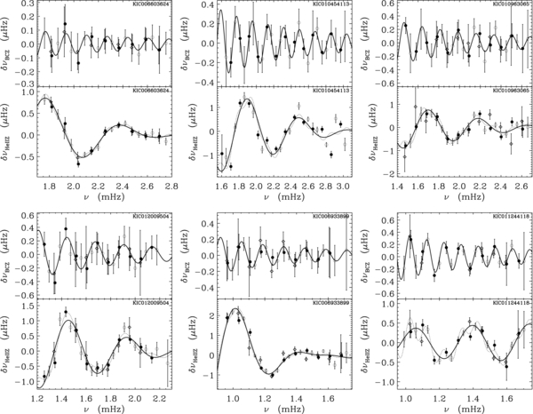
Figure 2. Illustration of method A: fits of Equations (A1) and (A2) to the residuals of frequencies of six Kepler stars (KIC numbers given in each panel) after removing a smooth component iteratively. The points correspond to l = 0 (black circles), l = 1 (open circles), and l = 2 (diamonds). The solid line is the best fit to the BCZ component (Equation (A1), upper panel for each star) and the HeIIZ component (Equation (A2), lower panel for each star). In the lower panels the dotted line shows the BCZ component superimposed on the HeIIZ component, as obtained separately and shown in the upper panel.
Download figure:
Standard image High-resolution image
Figure 3. Illustration of method B: fits of Equation (A6) to the second differences of the mean frequencies for eight Kepler stars (KIC numbers on the extreme left) and the histograms for the fitted values of τHeIIZ and τBCZ for different realizations of the data. The second differences of the frequencies of l = 0 (blue), l = 1 (red), and l = 2 (green) modes of the stars and their fit to Equation (A6) (black curve) are shown in the left panels. The corresponding histograms of the fitted values of τBCZ (in red) and τHeIIZ (in blue) for different realizations are shown in the right panels. The solid bands at the top of the right panels indicate the range of initial guesses for the two parameters in each fit.
Download figure:
Standard image High-resolution image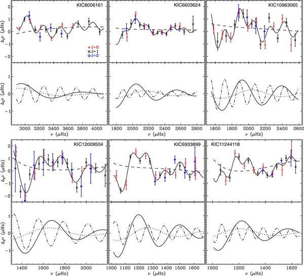
Figure 4. Illustration of method C: analyses results for six Kepler stars (KIC numbers given in each panel). The symbols in the upper panels denote second differences Δ2ν for low-degree modes. The solid curves are fits to Δ2ν based on the analysis by Houdek & Gough (2007, 2011). The dashed curves are the smooth contributions, including a third-order polynomial in  to represent the upper-glitch contribution from near-surface effects. The lower panels display the remaining individual contributions from the acoustic glitches to Δ2ν: the dotted and solid curves are the contributions from the first and second stages of helium ionization, and the dot-dashed curve is the contribution from the acoustic glitch at the base of the convective envelope.
Download figure:
Standard image High-resolution image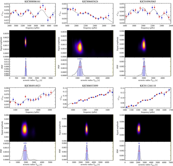
Figure 5. Illustration of method D: determination of TBCZ using frequency ratios for six Kepler targets. Each of the six panels corresponds to a target and is divided into three sub-panels. Top subpanels show the seismic variables ν*r010. Blue (red) dots with error bars are the observed values for ν*r01 (ν*r10). Solid lines show models (Equation (A19)) with the parameters corresponding to the highest posterior probabilities found by MCMC. Middle subpanels are two-dimensional probability functions in the plane (T, A). White (black) color corresponds to high (low) probability. Bottom subpanels show marginal probability distributions for the parameter T. Vertical blue lines indicate the medians of the distributions and hatched areas show the 68% level confidence intervals. Blue error bars, plotted above the peaks, are uncertainties deduced from these intervals, whereas red uncertainties, plotted across the peaks, are obtained by fitting the peaks with Gaussian profiles.
Download figure:
Standard image High-resolution imageWe compare the results for all 19 stars from all 4 methods in Table 2. The acoustic radii of the BCZ (TBCZ) determined by method D have been converted to acoustic depths (τBCZ) through the relation τBCZ = T0 − TBCZ = (2Δ0)−1 − TBCZ for comparison with the values determined by other methods. However, the uncertainties quoted for τBCZ from method D are the intrinsic uncertainties from the method, and do not include the uncertainties in T0. Method D did not consider the presence of the HeIIZ signal in the data.
Table 2. Comparison of Acoustic Depths of the Base of the Convective Envelope (τBCZ) and the Second Helium Ionization Zone (τHeIIZ) by Four Independent Methods
| KIC ID | T0 (s) | τBCZ (s) | τHeIIZ (s) | |||||
|---|---|---|---|---|---|---|---|---|
| Method A | Method B | Method C | Method D | Method A | Method B | Method C | ||
| KIC008006161* | 3353 ± 2 |  |
 |
 |
 |
⋅⋅⋅ |  |
 |
| KIC008379927 | 4170 ± 3 |  |
 |
 |
 |
⋅⋅⋅ |  |
 |
| KIC008760414 | 4273 ± 3 |  |
 |
 |
⋅⋅⋅ |  |
||
| KIC006603624* | 4549 ± 4 |  |
 |
 |
 |
 |
 |
 |
| KIC010454113* | 4757 ± 9 |  |
 |
 |
⋅⋅⋅ |  |
 |
 |
| KIC006106415 | 4821 ± 4 |  |
 |
 |
⋅⋅⋅ |  |
||
| KIC010963065* | 4882 ± 4 |  |
 |
 |
 |
 |
 |
 |
| KIC006116048 | 4985 ± 9 |  |
 |
 |
 |
 |
 |
 |
| KIC004914923* | 5662 ± 6 |  |
 |
 |
 |
⋅⋅⋅ |  |
 |
| KIC012009504* | 5701 ± 6 |  |
 |
 |
⋅⋅⋅ |  |
 |
 |
| KIC012258514 | 6711 ± 9 |  |
 |
⋅⋅⋅ |  |
 |
||
| KIC006933899* | 6963 ± 9 |  |
 |
 |
 |
 |
 |
 |
| KIC011244118* | 7012 ± 19 |  |
 |
 |
 |
 |
 |
 |
| KIC008228742 | 8116 ± 13 |  |
 |
 |
⋅⋅⋅ |  |
||
| KIC003632418 | 8264 ± 13 |  |
 |
 |
⋅⋅⋅ |  |
||
| KIC010018963 | 9057 ± 32 |  |
 |
⋅⋅⋅ | ⋅⋅⋅ |  |
||
| KIC007976303 | 9823 ± 38 |  |
 |
⋅⋅⋅ |  |
 |
||
| KIC011026764 | 9960 ± 19 |  |
 |
⋅⋅⋅ | ⋅⋅⋅ |  |
||
| KIC011395018 | 10548 ± 22 |  |
 |
⋅⋅⋅ | ⋅⋅⋅ |  |
||
Notes. 1In method D, the acoustic radius, TBCZ was determined, which has been converted to the corresponding acoustic depth, τBCZ using the T0 value derived from the average large separation, Δ0. 2A blank cell indicates that an estimation of the acoustic depth was not attempted, and a cell with "⋅⋅⋅" indicates that the estimated value did not pass the applied validity check for the relevant method. 3Values in parentheses denote a significant detection but not associated with an acoustic glitch. 4For KIC010454113, a secondary value of τBCZ ≈ 1850 s is obtained with lesser significance than the value quoted in methods B and C. *Stars illustrated in Figures 2–5.
Download table as: ASCIITypeset image
In Figure 6, we show the values of the acoustic depths obtained by different methods for all of the stars. A detailed comparison of the results follows in Section 5.1.
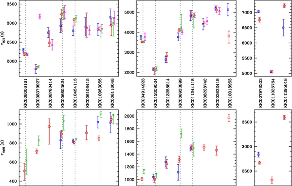
Figure 6. Comparison of acoustic depths τBCZ (upper panels) and τHeIIZ (lower panels) determined from the oscillatory signal in the Kepler frequencies of 19 stars by the four methods (blue empty squares for A, red empty circles B, green crosses C, and magenta empty triangles D). The stars have been grouped in three graphs for each glitch with different ranges according to their estimated values of τBCZ and τHeIIZ. The values from different methods for each star are slightly offset along the horizontal direction from the central positions for clarity. The gray dotted lines indicate the selected set of eight stars for which results are shown in Figures 2–5.
Download figure:
Standard image High-resolution image4. COMPARISON WITH STELLAR MODELS
The acoustic locations of the glitches determined by all of the methods described above do not depend on detailed modeling of the stars; they were derived purely from the observed frequencies. In order to check whether the estimated values of τBCZ and τHeIIZ are consistent with typical stellar models, we compared them with values from representative models of each star. In this, we adopted two approaches. The first one consisted of comparing the values with a broad family of models constructed to match the average seismic and spectroscopic properties of the stars to a fair extent. Additionally, we compared our values with the theoretical values of one optimally fitted model for each star.
For this exercise, we compared not the acoustic depths directly, but the fractional acoustic radii of the BCZ and the HeIIZ. This was done for two reasons. First, in a stellar model, the acoustic radius of a glitch, calculated from the center outward, is relatively free from the poorly known contribution to the sound speed from the outermost layers of the stars which lie above the glitch. Thus, it should theoretically be a more robust quantity than the acoustic depth, which, being calculated from the surface inward, would include the sound speed profile in the outer layers. However, in converting the acoustic depth estimated from the oscillatory signal in frequencies to the corresponding acoustic radius, we do use the approximate relationship between the total acoustic radius and the large separation. Second, by considering the fractional acoustic radii instead of the acoustic radii itself, we remove the effect of overall homology scaling of the models at slightly different masses and radii. Of course, the shift between the models in the relative position of the BCZ and the HeIIZ inside the star reflects a true departure of the models from the observed star.
4.1. Neighborhood Models
In this approach, we considered a broad family of theoretical models which mimic the global properties of the stars and their seismic properties, as listed in Table 1, but cannot be claimed to necessarily have frequencies that very closely match the observed ones. We deliberately spanned a very broad range in each of the global properties. This is because our aim here was to only determine the possible range in the locations of the acoustic glitches in stellar models similar to the target star, and compare the values estimated from the Kepler data. Further, we repeated the exact procedure of one of the methods (B) to obtain the acoustic depths τBCZ and τHeIIZ from the theoretical frequencies of the stellar models. This allowed us also to investigate possible systematic shifts between the theoretical acoustic locations of the glitches from the models and their estimated values from the oscillatory signal in the model frequencies themselves.
We used the Yale Stellar Evolution Code (YREC; Demarque et al. 2008) to model the stars. A detailed description of the models can be found in Appendix B. The first step of our modeling was to use the average large separation Δ0 and the frequency of maximum power, νmax, along with Teff and metallicity to determine the masses of the stars using a grid-based Yale-Birmingham pipeline (Basu et al. 2010; Gai et al. 2011). Mathur et al. (2012) have shown that grid-based estimates of stellar masses and radii agree very well with those obtained from more detailed modeling of the oscillation frequencies of stars, though with slightly lower precision (see also Silva Aguirre et al. 2011).
For each star, we specified 8–12 initial masses scanning a 2σ range on either side of the mass obtained by the grid modeling. For each initial mass, we modeled the star using three values of the mixing length parameter, α (1.826, 1.7, and 1.5; note that α = 1.826 is the solar calibrated value of α for YREC). For each value of mass and α, we assumed at least four different values of the initial helium abundance, Y0. In general, Y0 ranged from 0.25 to 0.30. The models were evolved from zero-age main sequence and the properties were output at short intervals to allow us to calculate oscillation frequencies for the model as it evolved.
All models satisfying the observed constraints on large separation, small separation, Teff, log g and [Fe/H] were selected for comparison. In order to get a reasonably large number of models, the uncertainty margin was assumed to be 2.0 μHz, 2.0 μHz, 200 K, 0.1 dex, and 0.1 dex, respectively. The number of models selected with these criteria ranged from about 80 to 800. For each of these models, the acoustic depths τBCZ and τHeIIZ were determined by a procedure exactly similar to method B adopted for the real data. The theoretically computed value of the frequency was taken as the mean value, and the uncertainty was adopted as that of the corresponding mode frequency in the Kepler data of the concerned star. Thus, the model data set mimicked the observed data set in terms of number of modes, specific modes used in the fitting, and the error bars on the frequencies.
The comparison of the fractional acoustic radii of the glitches in the models and our estimates from the Kepler data are shown in Figure 7 for two of the stars in our sample. One of them (KIC010963065) is a main-sequence star, while the other (KIC011244118) is in the subgiant phase. In this figure, we show the fractional acoustic radii of the glitches estimated from the Kepler data by method B along with the values obtained from the frequencies of the models by the same method, as described above. For the latter, the typical uncertainty (not shown in the graphs for the sake of clarity) would be similar to that of the values obtained from the Kepler data, since we have assumed the same uncertainties on the theoretical frequencies as the data. The acoustic depths obtained from the oscillatory signals have been converted to acoustic radii through the relation t = T0 − τ ≈ (2Δ0)−1 − τ. The error bars on the values from these methods include the uncertainty propagated in the calculation of T0 from Δ0, as listed in Table 2. The figure also shows the theoretical values of the fractional acoustic radii of the glitches from the models calculated using Equations (3) and (5). The two illustrated stars are typical of the sample. Results for other stars are similar to these with the discrepancies between the models and observations being either smaller or higher in a couple of stars.

Figure 7. Comparison of fractional acoustic radii TBCZ/T0 and THeIIZ/T0 determined from the oscillatory signal in the Kepler frequencies of two stars (KIC010963065 and KIC011244118) with corresponding values from representative models of the stars. In each case, the red empty circle with error bars represents the results from the data while the light gray dots represent the values determined from the calculated frequencies of the models. Method B was employed in both cases. The dark gray dots indicate the actual values of the fractional acoustic radii in the stellar models, calculated using Equations (3) and (5). For each star, the ranges of each axis shown in the graph correspond to ±1000 s and ±500 s of the values of TBCZ and THeIIZ determined from Kepler data, respectively.
Download figure:
Standard image High-resolution image4.2. Optimally Fitted Models
We also compared our estimated acoustic locations of the glitches to those in an optimally fitted model of each star. The fitted model was obtained through the Asteroseismic Modeling Portal (AMP; Metcalfe et al. 2009). The details of the stars studied here can be found in Mathur et al. (2012). Briefly, the models were obtained by optimizing the match between the observed frequencies and the modeled ones. To overcome the issue of the surface effects, we applied the empirical formula of Kjeldsen et al. (2008). The model acoustic radii were calculated as per the definitions given in Equation (3). The comparison of AMP model values of the fractional acoustic radii and those obtained from the four methods is shown in Figure 8.

Figure 8. Comparison of fractional acoustic radii TBCZ/T0 and THeIIZ/T0 determined from the oscillatory signal in the Kepler frequencies of 19 stars by the 4 methods (blue empty squares for A, red empty circles B, green crosses C, and magenta empty triangles D) and AMP model values (brown filled circles). For three stars, values obtained from independently fitted models made by the GARSTEC code are also shown (cyan starred symbol). The values from different methods for each star are slightly offset along the horizontal direction from the central positions for clarity. The gray dotted lines indicate the selected set of eight stars for which results are shown in Figures 2–5.
Download figure:
Standard image High-resolution image
For three of the stars, KIC008006161, KIC006106415, and KIC012009504, independent optimized models were made by fitting frequency ratios as described by Silva Aguirre et al. (2011, 2013). These models were constructed with the GARSTEC code (Weiss & Schlattl 2008), and are also shown in Figure 8.
5. DISCUSSION
5.1. Comparison between Methods and Uncertainties
Overall, we find remarkably good agreement between the values of the acoustic depths of the BCZ determined by different methods. In most cases, the τBCZ (or the corresponding TBCZ) agree with each other well within the quoted 1σ error bars (cf. Table 2 and Figure 6). In terms of relative uncertainties, the τBCZ and τHeIIZ values from different methods agree pairwise within 10% and 5%, respectively, for most of the stars.
The general agreement between τHeIIZ values from different methods is not as good as those for τBCZ, although it is mostly within 1σ uncertainties, and the values always match within 5% of each other. While comparing our estimates of the acoustic depths τBCZ and τHeIIZ from methods A, B, and C to the acoustic radii from method D, or from typical models, we invoked the relationship between the total acoustic radius T0 and the average large separation Δ0, i.e., T0 ≈ (2Δ0)−1. This relationship is an approximate one. Furthermore the observed average large separation, Δ0, depends on the adopted frequency range over which it is measured and on the adopted method.
Particular attention should be paid to the systematic biases involved in treating the outermost layers of the star by different seismic diagnostics dealing with the determination of acoustic depths of glitches. Although one may hope that the different methods (seismic diagnostics) will provide similar stellar radii, r, for the acoustic glitches of both the ionization zones of helium and the base of the surface convection zone, the seismically measured acoustic depths, τ(r), of these glitches will in general be different, for they depend on the very details of the adopted seismic diagnostic. For example, method C approximates the outer stellar layers by a polytrope with a polytropic index m = 3.5, allowing for some account of the location of the outer turning point of an incident acoustic wave by approximating the acoustic cutoff frequency, νac ≃ (m + 1)/τ (Houdek & Gough 2007). The location of the upper turning point affects the phase of an incident mode and consequently, also affects the location of the acoustic glitches, typically increasing their acoustic depths when the outer layers are approximated by a polytrope (Houdek & Gough 2007). A (mathematically) convenient way for estimating the phase at the upper turning point is to relate it to a fiducial location in the evanescent region far above the upper turning point, where the mode in the propagating region would "feel" the adiabatic sound speed, c, vanish, i.e., where c = 0. This location, lying well inside the evanescent zone of most of the acoustic modes, defines the acoustic radius or acoustic surface. The squared adiabatic sound speed, c2, decreases in the adiabatically stratified region of an outer convection zone nearly linearly with radius (e.g., Balmforth & Gough 1990; Gough 2013). The location of the acoustic radius can therefore be estimated where the linearly outward extrapolated c2, with respect to radius r, vanishes. In a solar model, the so-determined location of the seismic surface is about 111 s in acoustic height above the temperature minimum (Lopes & Gough 2001), or above 200 s in acoustic height above the photosphere (Monteiro et al. 1994; Houdek & Gough 2007). This shift may in part explain the differences between the location of the acoustic glitches between the stellar models and our seismically determined values.
There is also a noticeable systematic shift between the acoustic depth of the HeIIZ in a stellar model and its value estimated from the oscillatory signal in the model frequencies (see Figure 7). The fitted value of τHeIIZ, as obtained with methods A and B, is typically smaller than the model value by about 100 s, on average. However, we do not find such a systematic shift between the τBCZ values of the models and the fits. This is a general feature of most of the stars and might be because the depth of the He ii ionization zone cannot be uniquely defined since the ionization zone covers a finite range of radius. On the other hand, the base of the convection zone is a clearly defined layer within the star. Including the glitch contribution from the first stage of helium ionization in the seismic diagnostic, in addition to the contribution from the second stage of helium ionization, perhaps leads to a more accurate definition of the acoustic depth of helium ionization, as considered in method C, resulting in larger values for the fitted acoustic depth τHeIIZ as indicated in Table 2.
In Table 2 and Figures 7 and 8, we did not take account of these differences in the acoustic depths between the methods A–C and the calculated stellar models. It is also worth noticing that the T0 values of AMP models are systematically smaller (by about 300 s, or, by about 4%, on average) than those estimated from Δ0 of the Kepler data used in this paper (see Table 3). This may be due to a combination of factors, including imperfect modeling of the stars, especially of the surface layers. The AMP fitting has been subjected to the surface correction technique (Kjeldsen et al. 2008), while this was not included in the analysis of the present data. However, even with stellar models, a difference of up to 2% between the T0 values derived from the asymptotic relation (Equation (5)) and that from the large separation is expected (Hekker et al. 2013). Nevertheless, this contributes partially to the differences in the fractional acoustic radii of the glitches between AMP models and the estimates from the data. We have not estimated the uncertainties in the model values of the acoustic radii. Thus, it is difficult to make any quantitative comparison between these values and those obtained from the data.
Table 3. Acoustic Radii of Glitches in AMP Models
| KIC ID | TBCZa | THeIIZa | T0a | T0b |
|---|---|---|---|---|
| (s) | (s) | (s) | (s) | |
| KIC008006161* | 1177 | 2647 | 3239 | 3353 ± 2 |
| KIC008379927 | 1780 | 3285 | 4019 | 4170 ± 3 |
| KIC008760414 | 1675 | 3229 | 4084 | 4273 ± 3 |
| KIC006603624* | 1629 | 3503 | 4356 | 4549 ± 4 |
| KIC010454113* | 2326 | 3832 | 4611 | 4757 ± 9 |
| KIC006106415 | 2003 | 3735 | 4623 | 4821 ± 4 |
| KIC010963065* | 2128 | 3787 | 4673 | 4882 ± 4 |
| KIC006116048 | 2019 | 3844 | 4779 | 4985 ± 9 |
| KIC004914923* | 2177 | 4322 | 5410 | 5662 ± 6 |
| KIC012009504* | 2660 | 4485 | 5461 | 5701 ± 6 |
| KIC012258514 | 2761 | 5170 | 6410 | 6711 ± 9 |
| KIC006933899* | 2488 | 5188 | 6633 | 6963 ± 9 |
| KIC011244118* | 2286 | 5330 | 6726 | 7012 ± 19 |
| KIC008228742 | 3724 | 6278 | 7746 | 8116 ± 13 |
| KIC003632418 | 4289 | 6517 | 7911 | 8264 ± 13 |
| KIC010018963 | 4516 | 6992 | 8640 | 9057 ± 32 |
| KIC007976303 | 4012 | 7240 | 9305 | 9823 ± 38 |
| KIC011026764 | 3103 | 7303 | 9459 | 9960 ± 19 |
| KIC011395018 | 3363 | 7707 | 9954 | 10548 ± 22 |
Notes. Total acoustic radii of the stars in the AMP models and as estimated from the average large separation are also given. aCalculated from AMP model using Equations (3) and (5). bEstimated from Δ0 of Kepler data. *Stars illustrated in Figures 2–5.
Download table as: ASCIITypeset image
5.2. Discussion of Specific Stars
We further discuss the cases of the eight selected stars in detail below (ref. Figures 2–5). The cases of the 11 remaining stars are somewhat similar to these and a general understanding of the issues involved may be obtained from the selected subsample itself.
5.2.1. KIC008006161
This is a low-mass main-sequence star and one of the easiest cases for the determination of τBCZ or TBCZ, and all the methods converge to one consistent value which also agrees with the models. The determination of τHeIIZ from method A did not converge, and hence, is not included. Methods B and C agree with the model values, as well as the AMP and GARSTEC values.
5.2.2. KIC006603624
The oscillatory signal from the BCZ for this star seems to be substantially weaker in comparison to the signal from the HeIIZ, as borne out in each of Figures 2–5. In Figure 2, the amplitude of the oscillations in δνBCZ does not exceed 0.1 μHz, lower than all the other stars shown. It is, therefore, somewhat difficult to determine the acoustic location of the BCZ. This is reflected in the wider and flatter peaks in the histogram in method B (see Figure 3), the posterior probability distribution function (PDF) in method D (see Figure 5), and the larger error bars from all four methods. However, the median values of τBCZ derived from all of the methods agree quite well. The values of τHeIIZ obtained from methods A and B agree with each other, but only at the 2σ level with that from method C. The agreement with model values is barely at 1σ for TBCZ but well within 1σ for THeIIZ. The AMP model is also consistent with the other models.
5.2.3. KIC010454113
This star was attempted by the first three methods, and they produce consistent results for both BCZ and HeIIZ. The model values also lie close to these. This case illustrates the problem of aliasing encountered while fitting the oscillatory signal due to BCZ (see Appendix A.2). This is reflected in the dual peaks in the histogram of method B (Figure 3). Similarly, method C also finds a secondary value of τBCZ corresponding to the smaller peak from method B. We have considered the value with more numbers of Monte Carlo realizations as the true value of τBCZ.
5.2.4. KIC010963065
All four methods provide almost identical determinations of τBCZ (or corresponding TBCZ) but the τHeIIZ determined from method B agrees with those from the other two methods only at the 2σ level. However, the model values span the range of the determined THeIIZ (cf. Figures 7 and 8).
5.2.5. KIC004914923
The τBCZ values for this star have been obtained by all the methods, and the values agree within 1σ uncertainties. The PDF in method D shows a very small secondary peak at TBCZ ∼ 3000 s but the histogram for τBCZ in method B shows no such feature. The τHeIIZ could not be determined from method A, but both methods B and C provide values which agree within 2σ. The derived values for TBCZ and THeIIZ agree quite well with those derived from the model frequencies, as well as the AMP model values.
5.2.6. KIC012009504
Three methods, A–C, were applied for this star. Although in method B, we observed three peaks in the histogram for τBCZ, they cannot be explained as an aliasing artifact. Nevertheless, the highest peak value agrees very well with that from methods A and C. The τHeIIZ values obtained by the three methods are also consistent. However, the model values of TBCZ, as derived from both the AMP and GARSTEC models, seem to be smaller than our derived values, and actually correspond to the second highest peak in the histogram from method B. Given these facts, it is difficult to ascertain whether the discrepancy is because of inadequacy of the models to mimic the real star, or due to failure of our methods to detect the true oscillatory signal from the BCZ.
5.2.7. KIC006933899
The τBCZ values from all methods agree well within 1σ, as do the τHeIIZ determined from methods A and B. However, τHeIIZ from method C is more than 2σ deeper. While the model values of TBCZ agree very well with all of the derived values, the THeIIZ from methods A and B match the model fitted values while that from method C is close to the actual model value. The AMP model also lies in the vicinity of the other models.
5.2.8. KIC011244118
This is a relatively evolved star, for which there are possibly three mixed dipole modes. Once these modes are removed from consideration, all four methods produce exceptionally close median values of both τBCZ (TBCZ) and τHeIIZ (THeIIZ), even though the uncertainties are large in the former. The model fitted values have a larger scatter possibly because the radial orders of the mixed modes were not identical in such a wide range of models, and thus, those were not all removed during fitting.
5.2.9. Other Discrepant Cases
For the remaining 11 stars in the sample, the 4 methods agree remarkably well for most cases. Some discrepancies do occur for KIC008379927, KIC010018963, KIC007976303, and KIC011395018.
For KIC008379927, the first three methods produce consistent results for τBCZ. Method D does produce a pronounced peak in the PDF but at a value which is unlikely to correspond to the location of BCZ. A determination of τHeIIZ for this star was only possible from methods B and C which agree to within 1.5σ.
KIC010018963 seems to be a case where methods A and B have determined the mutually aliased values of τBCZ, and it is difficult to choose one over the other as the likely correct location of the BCZ.
KIC007976303 is an evolved star for which 23 frequencies could be used, and even some of these modes could be mixed in nature. Neither the τBCZ nor the τHeIIZ values determined from methods A and B agree for this star.
KIC011395018 is a subgiant star with several mixed modes, and it is therefore hardly surprising that methods A and B have failed to produce consistent values of τBCZ.
6. SUMMARY
We have used the oscillatory signal in the frequencies of 19 Kepler stars to determine the location of the 2 major acoustic glitches in the stellar interior, namely, the base of the convection zone and the second helium ionization zone. Four independent approaches were used which exploited either the presence of the signal in the frequencies themselves, the second differences of the frequencies or the ratio of small to the large separation. For the stars where more than one method was applied, we found remarkable agreement in the results, in general. There were, however, a few discrepant cases, some of which could be traced to the issue of aliasing between the acoustic depth and radius of the glitch. In some others, the presence of mixed modes prevented an accurate analysis.
As a check on the values of the acoustic radii of the acoustic glitches determined from the observed frequencies of a star, we also compared them with theoretical model values. For each star, a large number of representative models were constructed and the same method was applied for the theoretical frequencies of these as was done for the observed frequencies. For most of the stars, the estimated location of the glitches were found to be in close agreement with the model values, within error bars.
Although these results confirm the validity of the analysis done, the major result of the present work is to open the possibility of using the parameters of the glitches to perform model fitting. The proposed approach adds additional observational constraints, independent from other global and seismic parameters, that can be used in the process of finding the best possible model that reproduces the observations. Most important, these additional constraints can be the source for studying necessary improvements in the physics in order to ensure that all observables are fitted, as has been done for the Sun already (e.g., Christensen-Dalsgaard et al. 2011; Houdek & Gough 2011).
The present work demonstrates the viability of the techniques applied to determine the acoustic location of layers of sharp variation of sound speed in the stellar interior. These methods thus provide powerful tools for placing constraints on the stratification inside solar-type stars (Monteiro et al. 2002; Mazumdar 2005). With the availability of precise frequency sets for a large number of stars from the Kepler mission, one can use these techniques to follow the variation of the locations of acoustic glitches in a large ensemble of solar-type stars populating the main sequence and subgiant branches.
The amplitudes of the oscillatory signals from the acoustic glitches can also provide useful information about the stellar interior. The location as well as the strength of the glitch at the base of the convective envelope in cool stars can place independent constraints on the theories of convection(e.g., Christensen-Dalsgaard et al. 2011). Further, the amplitude of the oscillatory signal due to the second helium ionization zone can provide an estimate of the helium content in the stellar envelope (Pérez Hernández & Christensen-Dalsgaard 1998; Miglio et al. 2003; Basu et al. 2004; Monteiro & Thompson 2005; Houdek & Gough 2007).
We have demonstrated that the ratio τBCZ/T0 can be determined to an accuracy of a few percent. This ratio can be used to constrain Z and hence, may be able to distinguish between different heavy element mixtures. van Saders & Pinsonneault (2012) estimated that a variation in heavy element abundances by 0.1 dex can shift the acoustic depth by about 1% of the acoustic radius. Thus, with improved data from Kepler it should be possible to achieve the required accuracy to distinguish between different heavy element mixtures. There could be other effects which may also shift the acoustic depth of the convection zone and these systematic effects need to be studied before we can use asteroseismic data to study Z. Nevertheless, the variation that we find in τBCZ is consistent with that of van Saders & Pinsonneault (2012). In view of the large uncertainty in [Fe/H] and other stellar parameters, it is difficult to make a direct comparison with the predictions of van Saders & Pinsonneault (2012).
The analyses carried out here have obviously provided estimates of the amplitudes and other properties of the fits. The manner in which these reflect the stellar properties sensitively depends on the details of the fitting techniques and hence, unlike the acoustic locations, a direct comparison of those results of the different techniques is not meaningful. The interpretation of the results in terms of stellar properties will require detailed comparisons with the results of analysis of stellar model data, to be carried out individually for each technique. Such studies are envisaged as a follow-up to the present work.
Funding for the Kepler Discovery mission is provided by NASA's Science Mission Directorate. A.M. acknowledges support from the National Initiative on Undergraduate Science (NIUS) program of HBCSE (TIFR). S.B. acknowledges support from NSF grant AST-1105930. G.H. acknowledges support from the Austrian Science Fund (FWF) project P21205-N16. M.C. and M.J.P.F.G.M. acknowledge financial support from FCT/MCTES, Portugal, through the project PTDC/CTE-AST/098754/2008. M.C. is partially funded by POPH/FSE (EC). V.S.A. received financial support from the Excellence cluster "Origin and Structure of the Universe" (Garching). D.S. acknowledges the financial support from CNES. Funding for the Stellar Astrophysics Centre is provided by The Danish National Research Foundation. The research is supported by the ASTERISK project (ASTERoseismic Investigations with SONG and Kepler) funded by the European Research Council (grant agreement no.: 267864). N.C.A.R. is partially supported by the National Science Foundation. This work was partially supported by the NASA grant NNX12AE17G. This work has been supported, in part, by the European Commission under SPACEINN (grant agreement FP7-SPACE-2012-312844). J.B. acknowledges Othman Benomar for useful advice on MCMC methods. We thank Tim Bedding for suggesting improvements to the manuscript. We thank the anonymous referee for helping us to improve the paper.
APPENDIX A: METHODS FOR FITTING THE GLITCHES
We applied four different methods (labeled A–D) to determine the acoustic locations of the BCZ and the HeIIZ. Detailed descriptions of these methods are given in the following sections. In Figures 2–5, we illustrate each of the four methods, as applied to some Kepler stars.
A.1. Method A
In this method, the strategy is to isolate the signature of the acoustic glitches in the frequencies themselves. Compared to the methods involving second differences, described in Appendices A.2 and A.3, this has a different sensitivity to uncertainties (for a discussion on how the errors propagate in comparison with the uncertainties when using frequency combinations, please see the works by Ballot et al. 2004; Houdek & Gough 2007), does not require having frequencies of consecutive order and avoids the additional terms that need to be considered when fitting the expression to frequency differences. However, it is less robust on the convergence to a valid solution (the starting guess must be sufficiently close to the solution), since we do not put any constraints on what we consider to be a smooth component of the frequencies.
Here, we assume that only very low-degree data are available so that any dependence of the oscillatory signal on mode degree can be ignored. The expression for the signature due to the BCZ is taken from Monteiro et al. (1994), Christensen-Dalsgaard et al. (1995), and Monteiro et al. (2000). The expression for the signature due to the HeIIZ is from Monteiro & Thompson (1998) and Monteiro & Thompson (2005), with some minor adaptations and/or simplifications.
In the following, νr is a reference frequency, introduced for normalizing the amplitude. One good option would be to use νr = νmax (frequency of maximum power) but the actual value selected is not relevant unless we want to compare the amplitude of the signal of different stars.
The signal from the BCZ, after removing a smooth component from the frequencies, is written as (assuming there is no discontinuity in the temperature gradient at the BCZ)

The parameters to be determined in this expression are ABCZ, τBCZ, ϕBCZ for amplitude, acoustic depth, and phase, respectively. The typical values to expect for a star like the Sun are ABCZ ∼ 0.1 μHz, τBCZ ∼ 2300 s and ϕBCZ ∼ π/4.
The signal from HeIIZ, after removing a smooth component from the frequencies, is described by
The free parameters in this expression are  ,
,  , τHeIIZ, and ϕHeIIZ corresponding, respectively, to amplitude, acoustic width, acoustic depth, and phase. The typical values to expect for a solar-like star for these parameters are
  μHz,
μHz,  s, τHeIIZ ∼ 700 s, and ϕHeIIZ ∼ π/4. When performing the fitting of Equation (A2), leading to these parameters, it must be noted that the signature described by Equation (A1) is ignored and is treated as noise in the residuals.
If low-degree frequencies are used for a solar-type star, then the signals present in the data correspond to

or

Here, νsi (i = 1, 2) represents a "smooth" component of the mode frequency to be removed in the fitting. The parameters to fit these expressions are for Equation (A1) (BCZ): ABCZ, τBCZ, ϕBCZ; and for Equation (A2) (HeIIZ):  ,
,  , τHeIIZ, ϕHeIIZ. In this case, we treat δνBCZ as noise, since νs2 is treated as including νs1 and δνBCZ.
The fitting procedure used is the same method as described by Monteiro et al. (2000). This method uses an iterative process in order to remove the slowly varying trend of the frequencies, leaving the required signature given in either Equation (A1) or Equation (A2). A polynomial in n was fitted to the frequencies of all modes of given degree l separately using a regularized least-squares fit with third-derivative smoothing through a parameter, λ0 (see Monteiro et al. 1994 for the details). The residuals to those fits were then fitted for all degrees simultaneously. The latter fit is the "signal" either from the BCZ or from the HeIIZ. This procedure was then iterated (by decreasing the smoothing); at each iteration we removed from the frequencies the previously fitted signal and recalculated the smooth component of the frequencies, this time using the smaller value of λj (j = 1, 2, 3, ...). The iteration converged when the relative changes to the smooth component of the signal fell below 10−6 (typically this happened for j ≃ 3).
The initial smoothing, selected through the parameter λ0, defines the range of wavelengths whose variation we want to isolate. To isolate the signature from the BCZ, a smaller initial value of λ0 was required in order to ensure that the smooth component also extracts the signature from the HeIIZ. However, when isolating the signature from the HeIIZ, the shorter wavelength signature from the BCZ was also retained. We show the fits to Equations (A1) and (A2) in Figure 2 for six of the Kepler stars that we studied.
In order to estimate the impact on the fitting of the observational uncertainties, we used Monte Carlo simulations. We did so by producing sets of frequencies calculated from the observed values with added random values calculated from a standard normal distribution multiplied by the quoted observational uncertainty. In the fit, we removed frequencies with large uncertainties (>0.5 μHz for the BCZ and >1.0 μHz for the HeIIZ). For each star, we produced 500 sets of frequencies, determining the parameters as the standard deviation of the results for the parameters. Only valid fits were used as long as the number of valid fits represented more than 90% of the simulations. Otherwise, we considered that the signature had not been successfully fit (even if a solution could be found for the observations).
A.2. Method B
This method involves the second differences of the frequencies to determine τBCZ and τHeIIZ simultaneously by fitting a functional form to the oscillatory signals.
The oscillatory signal in the frequencies due to an acoustic glitch is quite small and is embedded in the frequencies together with a smooth trend arising from the regular variation of the sound speed in the stellar interior. It can be enhanced by using the second differences

instead of the frequencies ν(n, l) themselves (see, e.g., Gough 1990; Basu et al. 1994, 2004; Mazumdar & Antia 2001).
We fitted the second differences to a suitable function representing the oscillatory signals from the two acoustic glitches (Mazumdar & Antia 2001). We used the following functional form which has been adapted from Houdek & Gough (2007) (Equation (22) therein):
where a0, b2, c0, c2, τBCZ, ϕBCZ, τHeIIZ and ϕHeIIZ are eight free parameters of fitting. For one of the stars in our set (KIC010018963), we needed to use a slightly different function in which the constant term representing the smooth trend, a0, was replaced by a parabolic form: (a0 + a1ν + a2ν2). This was necessitated by the sensitivity of the fitted τ values to small perturbations to the input frequencies. The two τ values for the BCZ and the HeIIZ had uncertainties about 10 times larger (and overlapping) with the constant form, as compared to those with the parabolic form. Although this parabolic form could, in principle, be used for all stars as well, it actually interferes with the slowly varying periodic HeIIZ component in the limited range of observed frequencies and makes it difficult to determine τHeIIZ. Therefore, in adopting Equation (A6), we essentially assumed that the smooth trend in the frequencies had been reduced to a constant shift in the process of taking the second differences. We ignored frequencies which have uncertainties of more than 1 μHz.
While Equation (A6) is not the exact form prescribed by Houdek & Gough (2007), it captures the essential elements of that form while keeping the number of free parameters relatively small. The ignored terms can be shown to have relatively smaller contributions. We note that Basu et al. (2004) have shown that the exact form of the amplitudes of the oscillatory signal does not significantly affect the results (however, see also Houdek & Gough 2006). The fits of Equation (A6) to the second differences of some selected stars in our sample are shown in the left panels of Figure 3.
The fitting procedure is similar to the one described by Mazumdar et al. (2012). The fit was carried out through a nonlinear χ2 minimization, weighted by the uncertainties in the data. The correlation of uncertainties in the second differences was accounted for by defining the χ2 using a covariance matrix. The effects of the uncertainties were considered by repeating the fit for 1000 realizations of the data, produced by perturbing the frequencies by random uncertainties corresponding to a normal distribution with a standard deviation equal to the quoted 1σ uncertainty in the frequencies. The successful convergence of such a nonlinear fitting procedure is somewhat dependent on the choice of reasonable initial guesses. To remove the effect of initial guesses affecting the final fitted parameters, we carried out the fit for multiple combinations of starting values. For each realization, the fitting was repeated for 100 random combinations of initial guesses of the free parameters and the fit which produced the minimum value of χ2 was accepted.
The median value of each parameter for 1000 realizations was taken as its fitted value. The ±1σ uncertainty in the parameter was estimated from the range of values covering a 34% area about the median in the histogram of fitted values, assuming the error distribution to be Gaussian. Thus, the quoted uncertainties in these parameters reflect the width of these histograms on two sides of the median value. The histograms for τBCZ and τHeIIZ and the ranges of initial guesses of the corresponding parameters are shown in the right panels of Figure 3.
In some cases, the fitting of the τBCZ parameter suffers from the aliasing problem (Mazumdar & Antia 2001), where a significant fraction of the realizations are fitted with τBCZ equal to  . This becomes apparent from the histogram of τBCZ which appears bimodal with a reflection around T0/2 (e.g., for KIC010454113, shown in Figure 3). In such cases, we chose the higher peak in the histogram to represent the true value of τBCZ, and the uncertainty in the parameter was calculated after "folding" the histogram about the acoustic mid-point T0/2, where the acoustic radius was estimated from the mean large separation, Δ0. For a few stars, there are multiple peaks in the histogram for τBCZ, not all of which can be associated with the true depth of the BCZ or its aliased value (e.g., for KIC012009504, shown in the bottom right panel of Figure 3). In such cases, we chose only the most prominent peak to determine the median, and the uncertainty was estimated from the width of that peak. The remaining realizations were also neglected for estimating the other parameters such as τHeIIZ.
A.3. Method C
Approximate expressions for the frequency contributions, δνi, arising from acoustic glitches in solar-type stars were recently presented by Houdek & Gough (2007, 2011), which we adopt here for producing the results presented in Figure 4 and Table 2. A detailed discussion of the method can be found in those references; therefore, we present only a summary here. The complete expression for δνi is given by

where the terms on the right-hand side are the individual acoustic glitch components located at different depths inside the star.
The first component,
arises from the variation in γ1 induced by helium ionization. The constant m = 3.5 is a representative polytropic index in the expression for the approximate effective phase, ψ, appearing in the argument x = sgn(ψ)|3ψ/2|2/3 of the Airy function Ai(− x). We approximate ψ as

if  , and
, and

if  , in which
  , with
  II (I = II) being a phase constant, and τt is the location of the upper turning point of the mode. The location of the upper turning point of the oscillation mode is determined approximately from the polytropic representation of the acoustic cutoff frequency, leading to the expressions
 ![$\kappa (\tau)=[1-(m+1)^2/\omega ^2\tilde{\tau }^2]^{1/2}$](https://content.cld.iop.org/journals/0004-637X/782/1/18/revision1/apj489626ieqn131.gif) .
.
The coefficients associated with the glitch contribution from the first stage of helium ionization (He i) (first integral expression in Equation (A8)) are related to the coefficients of the second stage of helium ionization (He ii) by the constant ratios  ,
,  and
and  , where AII is the amplitude factor of the oscillatory He ii glitch component, ΔII is the acoustic width of the glitch, and τII ≡ τHeIIZ is its acoustic depth beneath the seismic surface. For the constant ratios
  ,
,  , and
, and  , we set the values at 0.45, 0.70, and 0.90, respectively, as did Houdek & Gough (2007, 2011). With this approach, the addition of the He i contribution does not introduce additional fitting coefficients in the seismic diagnostic (A8).
The second component in Equation (A7),
arises from the acoustic glitch at the base of the convection zone resulting from a near discontinuity (a true discontinuity in theoretical models using local mixing length theory with a non-zero mixing length at the lower boundary of the convection zone) in the second derivative of density. We model this acoustic glitch with a discontinuity in the squared acoustic cutoff frequency  at τBCZ, with Ac being proportional to the jump in
  , coupled with an exponential relaxation to a putative, glitch-free, model in the radiative zone beneath, with a relaxation time scale τ0 = 80 s, as did Houdek & Gough (2007, 2011). This leads to
where κc = κ(τBCZ) and  with c being a constant phase.
The additional upper-glitch component δuνi (i enumerates individual frequencies), which is produced, in part, by wave refraction in the stellar core, by the ionization of hydrogen and by the upper superadiabatic boundary layer of the envelope convection zone, is difficult to model. We approximate its contribution to Δ2ν as a series of inverse powers of ν, truncated at the cubic order:
The 11 coefficients ηα = (AII, ΔII, τHeIIZ, II, Ac, τBCZ, c, a0, a1, a2, a3), α = 1, ..., 11, were found by fitting the second differences (cf. Equation (A5)),
to the corresponding observations by minimizing
where  is the (i, j) element of the inverse of the covariance matrix C
 of the observational uncertainties in Δ2iν, computed, perforce, under the assumption that the uncertainties in the frequency data νi are independent. The covariance matrix Cηαγ of the uncertainties in the fitting coefficients ηα was established by Monte Carlo simulation.
Results for six of the stars in our sample are shown in Figure 4 in which the individual acoustic glitch contributions are illustrated in the lower panels.
A.4. Method D
Determinations of acoustic depths of glitches are biased by surface effects (e.g., Christensen-Dalsgaard et al. 1995). A way to remove such biases is to consider acoustic radii of the signatures. First, it is possible to perform posterior determinations of radii by comparing depths to the total acoustic radius of the star derived from the average large separation Δ0 (see Ballot et al. 2004); it is also possible to directly measure acoustic radii by considering the small separations d01 and d10 or the frequency ratios r01 and r10 as shown by Roxburgh & Vorontsov (2003).
We use the three-point differences:
and the corresponding ratios:
We denote the sets {d01, d10} and {r01, r10} by d010 and r010, respectively.
Using these variables, the main contributions of outer layers are removed (see Roxburgh 2005). The global trend of these variables then gives information on the core of the star (e.g., Silva Aguirre et al. 2011; Cunha & Brandão 2011). Nevertheless, the most internal glitches, such as the BCZ, also imprint their signatures over the global trend. Using solar data, Roxburgh (2009) showed that we can recover the acoustic radius of the BCZ (TBCZ) by the use of a Fourier transform on the residuals obtained after removing the global trend. As a consequence of this approach, information about surface layers, including He i and He ii ionization zones, are lost.
We used an approach similar to Roxburgh (2009) and develop a semi-automatic pipeline which extracts glitches from a frequency table of l = 0 and 1 modes. Instead of fitting a background first, then making a Fourier transform, we do both simultaneously by fitting the variable y = ν*r010 (or y = ν*d010) with the following expression:
where ν* = ν/νr and νr is a reference frequency. We have m + 3 free parameters: {ck}, A, T, and ϕ.
To be able to estimate reliable uncertainties for TBCZ, we performed a Markov Chain Monte Carlo (MCMC) to fit the data. Our MCMC fitting algorithm is close to the one described, for example, in Benomar et al. (2009) or Handberg & Campante (2011), but without parallel tempering. Moreover, in our case, the noise is not multiplicative and exponential but additive and normal. We fixed m = 2 and νr = 0.8νmax, similar to the value adopted for the Sun by Roxburgh (2009). We used uniform priors for A, T, and ϕ. The prior for A was very broad (between 0 and 10max (|y|)); ϕ was 2π-periodic with a uniform prior over [0, 2π], and T was restricted to [δT, T0 − δT], where δT = (max (ν) − min (ν))−1. To determine priors for {ck}, we first performed a standard linear least-square fitting without including the oscillatory component. Once we obtained the fitted values,  , and associated uncertainties, σk, we used for ck priors which are uniform over
 ![$[\tilde{c}_k- 3\sigma _k,\tilde{c}_k+ 3\sigma _k]$](https://content.cld.iop.org/journals/0004-637X/782/1/18/revision1/apj489626ieqn144.gif) with Gaussian decay around this interval. After a 200,000-iteration learning phase (the learning method we used is based on Benomar et al. 2009), MCMC was run for 107 iterations. We tested the convergence by verifying the consistence of results obtained by using the first and second half of the chain.
with Gaussian decay around this interval. After a 200,000-iteration learning phase (the learning method we used is based on Benomar et al. 2009), MCMC was run for 107 iterations. We tested the convergence by verifying the consistence of results obtained by using the first and second half of the chain.
Posterior PDFs for T are plotted for different stars in Figure 5. Some PDFs exhibit a unique and clear mode that we attributed to the BCZ. TBCZ was then estimated as the median of the distribution and 1σ error bars were taken as a 68% confidence limit of the PDF. Nevertheless, some other PDFs exhibit other small peaks. They can be due to noise but also can be due to other glitch signatures present in the data, especially tiny residuals from the outer layers. To take care of such situations, we also computed TBCZ by isolating the highest peak and fitting it with a Gaussian profile. When the secondary peaks are small enough, the values and associated uncertainties obtained through the two methods are very similar. We have been successful mainly on main-sequence stars, while subgiant stars presenting mixed modes strongly disturb the analysis.
APPENDIX B: DETAILS OF YREC STELLAR MODELS
The input physics for the YREC models included the OPAL equation of state (Rogers & Nayfonov 2002) and the OPAL high-temperature opacities (Iglesias & Rogers 1996) supplemented with low-temperature opacities from Ferguson et al. (2005). All nuclear reaction rates were from Adelberger et al. (1998), except for the rate of the 14N(p, γ)15O reaction, which was fixed at the value of Formicola et al. (2004). Core overshoot of 0.2Hp was included where relevant. For the stars that did not have very low metallicities, we included the diffusion and settling of helium and heavy elements. This was done as per the prescription of Thoul et al. (1994).
We use four grids for this: the models from the Yonsei-Yale isochrones (Demarque et al. 2004), and the grids of Dotter et al. (2008), Marigo et al. (2008), and Gai et al. (2011).